REVIEW 2 major objections 6 minor 61 references
Stacked linear combinations of unitaries give a single dial that trades barren plateaus against classical simulability.
Reviewed by Pith at T0; open to challenge. T0 means a machine referee read the full paper against a public rubric. the ladder, T0–T4 →
T0 review · grok-4.5
2026-07-31 07:51 UTC pith:UAN2HD6P
load-bearing objection Solid stacked-LCU construction and FF variance proof; the tunable-trainability claim is real for unnormalised m but still open for the postselected objective people actually optimise. the 2 major comments →
Stacking the Deck: Tunable Trainability in Stacked LCUs
The pith
A machine-rendered reading of the paper's core claim, the machinery that carries it, and where it could break.
Core claim
An S-LCU of l layers, each an LCU of k fermionic Gaussian unitaries, yields a loss-landscape variance bounded from below by Ω(1/(n k^{3l})) for traceless quadratic observables, while direct classical simulation of the expanded state costs O(k^{2l} n³) and the coherent quantum circuit uses only O(l k n²) gates before post-selection. The layer count l is therefore a single dial that trades classical hardness against the rate of cost concentration.
What carries the argument
A diagrammatic moment calculation that expresses the first and second moments of the S-LCU cost through the Gram matrix of an overcomplete frame built from the first- and second-order commutants of the underlying compact group; for free fermions this Gram matrix is evaluated explicitly and raised to the l-th power.
Load-bearing premise
The claimed classical–quantum gap treats direct expansion of the Gaussian-rank superposition as the relevant classical cost and counts only coherent gates on the quantum side, setting aside post-selection overhead and any classical algorithm that might exploit the stacked product structure.
What would settle it
Exhibit either a classical algorithm that evaluates local expectations of an l-layer free-fermion S-LCU faster than O(k^{2l} n³), or a concrete instance where the measured cost variance falls below the stated Ω(1/(n k^{3l})) lower bound for traceless quadratic observables.
If this is right
- Fixing the layer count rules out exponential barren plateaus in both qubit number and terms-per-layer for free-fermion S-LCUs.
- Increasing layers produces an arbitrarily high polynomial separation (in k) between expanded classical cost and coherent quantum gate count.
- The same diagrammatic commutant method applies to any compact group whose low-order commutants are known, giving a template for other ansatz families.
- Staged or warm-start training that grows layers or terms incrementally is suggested as a practical way to keep early gradients large.
Where Pith is reading between the lines
- If post-selection or amplitude amplification can be controlled without spoiling the polynomial gap, free-fermion S-LCUs become a concrete candidate for near-term quantum advantage in fermionic simulation tasks.
- The construction suggests a broader design pattern: start from any classically easy, plateau-free family and stack LCUs until the desired classical hardness is reached.
- Measuring how variance and success probability jointly scale under realistic noise would immediately test whether the theoretical dial remains usable on hardware.
Editorial analysis
A structured set of objections, weighed in public.
Referee Report
Summary. The manuscript introduces a stacked linear-combination-of-unitaries (S-LCU) variational ansatz: l sequentially applied LCUs, each containing k unitaries on n qubits. For unitaries sampled Haar-randomly from a compact group and coefficients sampled uniformly from a Dirichlet distribution, the authors derive first- and second-moment formulas for the unnormalised expectation m=tr(ρO). The second moment is expressed through powers of a Dirichlet-weighted Gram matrix associated with an overcomplete commutant frame. Specialising to fermionic Gaussian unitaries, the paper computes the relevant Gram matrix and proves, for a computational-basis input and normalised traceless quadratic observable, Var[m] ≥ Ω(1/(n k^{3l})). It compares direct Gaussian-rank term-expansion simulation, quoted at O(k^{2l}n^3), with an O(lkn^2) coherent quantum gate count, while deferring postselection overhead and improved structure-aware classical methods.
Significance. If the analysis stands, the work supplies a concrete, parameter-free mechanism for dialing between polynomial loss-concentration bounds and the cost of a natural classical term-expansion simulation. Particularly valuable are the explicit commutant-projector and Dirichlet-moment derivations, the use of powers of an overcomplete Gram frame rather than a Weingarten inverse, the explicit free-fermion Gram matrix, and a general second-moment formula with a controlled remainder. These results could be useful beyond the present ansatz. The broader practical significance remains conditional on the treatment of postselection and on the absence of a classical algorithm that exploits stacking more efficiently.
major comments (2)
- [§II, §IV.B, Theorem 1] §II Eqs. (2)–(4), §IV.B after Eq. (57), and Theorem 1: the variance bound applies to the unnormalised cost m. In a postselected LCU experiment, however, the conditional objective normally estimated and optimised is m/p_s. Result 1 with O=I gives E[p_s]=(2/(k+1))^l, so adding layers also exponentially suppresses the success probability for k≥2. No anticoncentration or joint moment bound here transfers the lower bound on Var[m] to Var[m/p_s], its gradients, or the shot cost of estimating them. The statement that the calculation "accounts for" postselection is true only for m as defined. Please either analyse the normalised objective/sample complexity or explicitly restrict the trainability claims to the success-weighted objective.
- [§IV.B, Result 3] §IV.B Eqs. (56)–(57), Result 3, the abstract, and §VI: O(k^{2l}n^3) is an upper bound for direct pairwise Gaussian-rank term expansion, not a classical lower bound, and the manuscript explicitly says it knows no structure-aware improvement. Likewise, O(lkn^2) is a coherent gate count before postselection or amplification. These two upper bounds therefore do not by themselves establish an end-to-end classical–quantum time separation. The abstract and Result 3 should consistently describe the comparison as relative to the named direct term-expansion method, or else supply a tighter state-of-the-art/lower-bound argument and include the relevant quantum overhead.
minor comments (6)
- [§III, §IV.A] §III opening and §IV.A: a polynomial lower bound on cost variance does not by itself imply a corresponding lower bound on gradient variance unless the conditions invoked from Ref. [21] are verified. The manuscript generally says "diagnostic," but a few surrounding statements about barren plateaus/trainability should keep this distinction explicit.
- [§VI and Appendix F] §VI versus Result 4: the conclusion calls the arbitrary-state/observable formula "exact," while Result 4 includes an O(l2^{-n}tr(O^2)) remainder. Either retain the finite Δ/sum over R^r explicitly or describe Result 4 as an explicit formula with a controlled, exponentially small error.
- [§IV.3] §IV.3: the displayed Gram matrix is difficult to audit because the full ordered-frame index map is implicit, while Appendix E refers to indices such as G_{3,7}. Please state the block ordering and dimensions explicitly in the main text.
- [§IV.4, Eq. (54)] Eq. (54): saying that the observable vector is obtained by replacing ρ0 by O is ambiguous for entries containing ρ0^2 or Pρ0Pρ0. Please give the componentwise replacement rule.
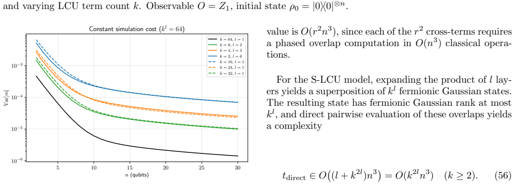
- [Figure 2] Figure 2: the caption says configurations have constant expanded count k^l=64, but the dashed l=1 comparator curves use k=16, 24, and 32. Please clarify that these are comparators rather than constant-count configurations and explain their selection.
- [Figure 1] Figure 1: please state whether the plotted curves are exact evaluations from Result 2 rather than sampled estimates, and consider overlaying the Theorem 1 lower-bound scaling for the plotted parameters.
Circularity Check
No significant circularity: variance bound and complexity trade-off are derived in-paper from Haar/Dirichlet moments and commutant Gram matrices.
full rationale
The central claims (Result 1–3, Theorem 1) are obtained by an explicit diagrammatic moment calculation: unbalanced Haar moments vanish (Lemma 1), Dirichlet coefficient moments are elementary (Appendix G), the layer operator is expanded into three pairing projectors, and the second moment is the contraction of the powered Dirichlet-weighted Gram matrix of the free-fermion commutant frame (Result 2, Appendices E–F). The lower bound Var[m] ≥ (k E[a⁴_i])^l /(2n−1) follows by dropping non-negative first-order-block terms under the stated hypotheses on O and ρ₀ (Theorem 2 → Theorem 1). Classical O(k^{2l} n³) and quantum O(l k n²) counts are standard Gaussian-rank and matchgate gate-count arguments, not fitted or self-defined. Citation [19] (authors’ prior single-LCU trainability paper) and external commutant bases (Diaz et al., matchgate literature) supply motivation and known algebraic ingredients; they are not inverted or renamed into the stacked variance formula. No parameter is fitted to data and re-presented as a prediction; no uniqueness theorem is imported to forbid alternatives. Scope caveats (unnormalised m vs postselected m/p_s; direct vs structure-aware classical simulation) affect correctness risk, not circularity of the derivation chain.
Axiom & Free-Parameter Ledger
axioms (6)
- domain assumption Unitaries in each LCU term are i.i.d. Haar on a compact group G (here U(1)×Spin(2n)) and coefficients are i.i.d. uniform Dirichlet; moments are taken over that product measure.
- standard math Lemma 1: unbalanced Haar moments E[U^{⊗a} ⊗ U^{*⊗b}] vanish when G contains a scalar ωI with ω^{a-b}≠1.
- domain assumption First- and second-order commutants of fermionic Gaussian unitaries are spanned by {I,P}/√d and the {Q0_κ, Q1_κ} family of Diaz et al. / matchgate literature.
- domain assumption Direct classical simulation cost of a fermionic Gaussian-rank-r state is O(r² n³) via pairwise phased overlaps; S-LCU expansion gives r≤k^l.
- domain assumption Variance of the unnormalized cost m=tr(ρO) is a valid trainability diagnostic (cost concentration implies barren plateaus under Arrasmith et al. conditions).
- standard math Uniform Dirichlet moments E[a_i²]=2/(k(k+1)), E[a_i⁴]=24/(k(k+1)(k+2)(k+3)), E[a_i² a_j²]=4/(k(k+1)(k+2)(k+3)).
invented entities (1)
-
Stacked LCU (S-LCU) / Free Fermion S-LCU ansatz
independent evidence
read the original abstract
Variational quantum circuits have been central to many proposed near-term applications of quantum computing, but a growing body of evidence suggests that trainability and quantum advantage are fundamentally at odds: ans\"atze expressive enough to resist efficient classical simulation tend to exhibit barren plateaus, while structures that provably rule out barren plateaus typically render them classically simulable. We propose a stacked linear combination of unitaries (S-LCU) as a variational ansatz which provides a tunable trade-off between barren plateaus and classical simulability. Using a diagrammatic analysis, we bound the loss-landscape variance of the Free Fermion S-LCU, whose elements are fermionic Gaussian unitaries. We prove a variance lower bound of $\Omega(1/(n k^{3l}))$, with a simulation cost of $O(k^{2l} n^3)$ using the best known classical algorithm, compared to a quantum gate complexity of only $O(lkn^2)$. The number of layers $l$ serves as a single dial that trades computational complexity against the rate of cost concentration. This offers practitioners a systematic method for constructing ans\"atze with a complexity-trainability trade-off that best suits their application and hardware.
Figures

Reference graph
Works this paper leans on
-
[1]
It is spanned by the orthonormal basis I√ d , P√ d = 1√ d · , 1√ d · P , d= 2 n
First-Order Commutant The first-order commutant of the group of fermionic Gaussian unitaries is well-studied [26, 30, 31]. It is spanned by the orthonormal basis I√ d , P√ d = 1√ d · , 1√ d · P , d= 2 n. (47) HerePis theparityoperator, defined as P:=Z ⊗n = (−i)n ·c 1c2 . . . c2n.(48) 6
-
[2]
[30, 31]: ( Q0 κ )2n κ=0 ∪ ( Q1 κ )2n κ=0 ,(49) where Q0 κ :=N κ X s∈( [2n] κ ) cs ⊗c s,(50) Q1 κ :=i κmod 2 · Q0 κ P ,(51) where [2n] κ :={s⊆[2n] :|s|=κ}andN κ := 2n q2n κ −1
Second-Order Commutant We use the definition of the second-order commutant from Diazet al.[26], which has also been characterised in Refs. [30, 31]: ( Q0 κ )2n κ=0 ∪ ( Q1 κ )2n κ=0 ,(49) where Q0 κ :=N κ X s∈( [2n] κ ) cs ⊗c s,(50) Q1 κ :=i κmod 2 · Q0 κ P ,(51) where [2n] κ :={s⊆[2n] :|s|=κ}andN κ := 2n q2n κ −1 . Algebraically, the second line isQ 1 κ =...
-
[3]
(37), is given below
Gram Matrix The full Gram matrixGfor the FF-S-LCU, expressed in the ordered framePdefined in Eq. (37), is given below. We define the following shorthand: νκ := q2n κ d , σ κ := (−1)⌊κ/2⌋,(52) ϵκ := (−1)κ(κ+1)/2.(53) whered= 2 n. Derivations for each scalar element of the matrix are provided in Appendix E. Q0κ Q1κ P P P P P P P P Q0κ δκ,κ′ · · · · · · · · ...
-
[4]
Projections of Initial State and Observable Result 2 contracts the layer operator with the initial state and observable. The initial state boundary vector needed for this contraction has entries 1 d h tr(ρ0)2,tr(P ρ0) tr(ρ0),tr(P ρ0) tr(ρ0), tr(P ρ0)2,tr(ρ 2 0),tr(P ρ2 0),tr(P ρ2 0), tr(P ρ0P ρ0), ePκ(ρ0), eCκ(ρ0) i (54) where ePκ(ρ0) := tr(ρ⊗2 0 Q0 κ), e...
-
[5]
Benedetti, E
M. Benedetti, E. Lloyd, S. Sack, and M. Fiorentini, Pa- rameterized quantum circuits as machine learning mod- els, Quantum Science and Technology4, 043001 (2019)
2019
-
[6]
Biamonte, P
J. Biamonte, P. Wittek, N. Pancotti, P. Rebentrost, N. Wiebe, and S. Lloyd, Quantum machine learning, Na- ture549, 195 (2017). 9
2017
-
[7]
Peruzzo, J
A. Peruzzo, J. McClean, P. Shadbolt, M.-H. Yung, X.-Q. Zhou, P. J. Love, A. Aspuru-Guzik, and J. L. O’Brien, A variational eigenvalue solver on a photonic quantum processor, Nature Communications5, 4213 (2014)
2014
-
[8]
J. R. McClean, J. Romero, R. Babbush, and A. Aspuru- Guzik, The theory of variational hybrid quantum- classical algorithms, New Journal of Physics18, 023023 (2016)
2016
-
[9]
Tilly, H
J. Tilly, H. Chen, S. Cao, D. Picozzi, K. Setia, Y. Li, E. Grant, L. Wossnig, I. Rungger, G. G. Booth, and J. Tennyson, The variational quantum eigensolver: A re- view of methods and best practices, Physics Reports986, 1 (2022)
2022
-
[10]
E. Farhi, J. Goldstone, and S. Gutmann, A quan- tum approximate optimization algorithm (2014), arXiv:1411.4028 [quant-ph]
Pith/arXiv arXiv 2014
-
[11]
Blekos, D
K. Blekos, D. Brand, A. Ceschini, C.-H. Chou, R.-H. Li, K. Pandya, and A. Summer, A review on Quantum Approximate Optimization Algorithm and its variants, Physics Reports1068, 1 (2024)
2024
-
[12]
Abbas, A
A. Abbas, A. Ambainis, B. Augustino,et al., Challenges and opportunities in quantum optimization, Nature Re- views Physics6, 718 (2024)
2024
-
[13]
J. R. McClean, S. Boixo, V. N. Smelyanskiy, R. Bab- bush, and H. Neven, Barren plateaus in quantum neural network training landscapes, Nature Communications9, 4812 (2018)
2018
-
[14]
Cerezo, A
M. Cerezo, A. Sone, T. Volkoff, L. Cincio, and P. J. Coles, Cost function dependent barren plateaus in shal- low parametrized quantum circuits, Nature Communica- tions12, 1791 (2021)
2021
-
[15]
Larocca, S
M. Larocca, S. Thanasilp, S. Wang, K. Sharma, J. Bia- monte, P. J. Coles, L. Cincio, J. R. McClean, Z. Holmes, and M. Cerezo, Barren plateaus in variational quantum computing, Nature Reviews Physics7, 174–189 (2025)
2025
-
[16]
M. Cerezo, M. Larocca, D. Garc ´ ıa-Mart ´ ın, N. L. Diaz, P. Braccia, E. Fontana, M. S. Rudolph, P. Bermejo, A. Ijaz, S. Thanasilp, E. R. Anschuetz, and Z. Holmes, Does provable absence of barren plateaus imply classical simulability?, arXiv preprint arXiv:2312.09121 (2023)
Pith/arXiv arXiv 2023
-
[17]
A. M. Childs and N. Wiebe, Hamiltonian Simula- tion Using Linear Combinations of Unitary Oper- ations, Quantum Information and Computation12, 10.26421/qic12.11-12 (2012)
-
[18]
N. Khatri, G. Matos, L. Coopmans, and S. Clark, Quixer: A quantum transformer model, arXiv preprint arXiv:2406.04305 (2024)
Pith/arXiv arXiv 2024
-
[19]
Heredge, M
J. Heredge, M. West, L. Hollenberg, and M. Sevior, Nonunitary quantum machine learning, Phys. Rev. Appl. 23, 044046 (2025)
2025
-
[20]
Coopmans and M
L. Coopmans and M. Benedetti, On the sample complex- ity of quantum Boltzmann machine learning, Communi- cations Physics7, 274 (2024)
2024
-
[21]
H. Yao, X. Liu, M. Jing, G. Li, and X. Wang, LCQNN: Linear combination of quantum neural networks, arXiv preprint arXiv:2507.02832 (2025)
Pith/arXiv arXiv 2025
-
[22]
Coyle, S
B. Coyle, S. Raj, N. Mathur, E. A. Cherrat, N. Jain, S. Kazdaghli, and I. Kerenidis, Training-efficient density quantum machine learning, npj Quantum Information 11, 172 (2025)
2025
-
[23]
N. Khatri, S. Zohren, and G. Matos, Trainability of parametrised linear combinations of unitaries, arXiv preprint arXiv:2506.22310 (2025)
Pith/arXiv arXiv 2025
-
[24]
Dias and R
B. Dias and R. K¨ onig, Classical simulation of non- Gaussian fermionic circuits, Quantum8, 1350 (2024)
2024
-
[25]
Arrasmith, Z
A. Arrasmith, Z. Holmes, M. Cerezo, and P. J. Coles, Equivalence of quantum barren plateaus to cost concen- tration and narrow gorges, Quantum Science and Tech- nology7, 045015 (2022)
2022
-
[26]
A. A. Mele, Introduction to Haar measure tools in quan- tum information: A beginner’s tutorial, Quantum8, 1340 (2024)
2024
-
[27]
L. G. Valiant, Quantum computers that can be simu- lated classically in polynomial time, inProceedings of the Thirty-Third Annual ACM Symposium on Theory of Computing(ACM, 2001) pp. 114–123
2001
-
[28]
B. M. Terhal and D. P. DiVincenzo, Classical simulation of noninteracting-fermion quantum circuits, Physical Re- view A65, 032325 (2002)
2002
-
[29]
Matos, C
G. Matos, C. N. Self, Z. Papi´ c, K. Meichanetzidis, and H. Dreyer, Characterization of variational quantum algo- rithms using free fermions, Quantum7, 966 (2023)
2023
-
[30]
N. Diaz, D. Garc ´ ıa-Mart ´ ın, S. Kazi, M. Larocca, and M. Cerezo, Showcasing a barren plateau the- ory beyond the dynamical lie algebra, arXiv preprint arXiv:2310.11505 (2023)
Pith/arXiv arXiv 2023
-
[31]
Fontana, D
E. Fontana, D. Herman, S. Chakrabarti, N. Kumar, R. Yalovetzky, J. Heredge, S. H. Sureshbabu, and M. Pis- toia, Characterizing barren plateaus in quantum ans¨ atze with the adjoint representation, Nature Communications 15, 7171 (2024)
2024
-
[32]
K¨ okc¨ u, T
E. K¨ okc¨ u, T. Steckmann, Y. Wang, J. K. Freericks, E. F. Dumitrescu, and A. F. Kemper, Fixed depth hamilto- nian simulation via cartan decomposition, Physical Re- view Letters129, 070501 (2022)
2022
-
[33]
Wiersema, E
R. Wiersema, E. K¨ okc¨ u, A. F. Kemper, and B. N. Bakalov, Classification of dynamical lie algebras for translation-invariant 2-local spin systems in one dimen- sion, npj Quantum Information10, 110 (2024)
2024
-
[34]
P. Sierant, X. Turkeshi, and P. S. Tarabunga, The- ory of the matchgate commutant, arXiv preprint arXiv:2603.12392 (2026)
arXiv 2026
-
[35]
M. Lastres and S. Moudgalya, Geometry of free fermion commutants, arXiv preprint arXiv:2604.05031 (2026)
Pith/arXiv arXiv 2026
-
[36]
Reardon-Smith, M
O. Reardon-Smith, M. Oszmaniec, and K. Korzekwa, Im- proved simulation of quantum circuits dominated by free fermionic operations, Quantum8, 1549 (2024)
2024
-
[37]
J. Cudby and S. Strelchuk, Gaussian decomposition of magic states for matchgate computations, arXiv preprint arXiv:2307.12654 (2024)
Pith/arXiv arXiv 2024
-
[38]
Babbush, C
R. Babbush, C. Gidney, D. W. Berry, N. Wiebe, J. Mc- Clean, A. Paler, A. Fowler, and H. Neven, Encoding elec- tronic spectra in quantum circuits with linear T complex- ity, Physical Review X8, 041015 (2018)
2018
-
[39]
D. W. Berry, A. M. Childs, R. Cleve, R. Kothari, and R. D. Somma, Simulating Hamiltonian dynamics with a truncated Taylor series, Physical Review Letters114, 090502 (2015)
2015
-
[40]
Kieferov´ a, A
M. Kieferov´ a, A. Scherer, and D. W. Berry, Simulat- ing the dynamics of time-dependent Hamiltonians with a truncated Dyson series, Physical Review A99, 042314 (2019)
2019
-
[41]
G. H. Low, V. Kliuchnikov, and N. Wiebe, Well- conditioned multiproduct Hamiltonian simulation (2019), arXiv:1907.11679 [quant-ph]
Pith/arXiv arXiv 2019
-
[42]
Gily´ en, Y
A. Gily´ en, Y. Su, G. H. Low, and N. Wiebe, Quantum singular value transformation and beyond: Exponential improvements for quantum matrix arithmetics, inPro- 10 ceedings of the 51st Annual ACM SIGACT Symposium on Theory of Computing(2019) pp. 193–204
2019
-
[43]
Chakraborty, A
S. Chakraborty, A. Gily´ en, and S. Jeffery, The power of block-encoded matrix powers: Improved regression tech- niques via faster Hamiltonian simulation, in46th Inter- national Colloquium on Automata, Languages, and Pro- gramming (ICALP 2019), Vol. 132 (2019) pp. 33:1–33:14
2019
-
[44]
Skolik, J
A. Skolik, J. R. McClean, M. Mohseni, P. van der Smagt, and M. Leib, Layerwise learning for quantum neural net- works, Quantum Machine Intelligence3, 5 (2021)
2021
-
[45]
H. R. Grimsley, S. E. Economou, E. Barnes, and N. J. Mayhall, An adaptive variational algorithm for exact molecular simulations on a quantum computer, Nature Communications10, 3007 (2019)
2019
-
[46]
Penrose, Applications of negative dimensional ten- sors, inCombinatorial Mathematics and its Applications, edited by D
R. Penrose, Applications of negative dimensional ten- sors, inCombinatorial Mathematics and its Applications, edited by D. J. A. Welsh (Academic Press, 1971) pp. 221–244
1971
-
[47]
Abramsky and B
S. Abramsky and B. Coecke, A categorical semantics of quantum protocols, inProceedings of the 19th Annual IEEE Symposium on Logic in Computer Science (LICS) (IEEE, 2004) pp. 415–425
2004
-
[48]
Coecke and A
B. Coecke and A. Kissinger,Picturing Quantum Pro- cesses: A First Course in Quantum Theory and Di- agrammatic Reasoning(Cambridge University Press, 2017)
2017
-
[49]
J. Biamonte and V. Bergholm, Tensor networks in a nut- shell, arXiv preprint arXiv:1708.00006 (2017)
Pith/arXiv arXiv 2017
-
[50]
Weingarten, Asymptotic behavior of group integrals in the limit of infinite rank, Journal of Mathematical Physics19, 999 (1978)
D. Weingarten, Asymptotic behavior of group integrals in the limit of infinite rank, Journal of Mathematical Physics19, 999 (1978)
1978
-
[51]
B. Collins, Moments and cumulants of polynomial ran- dom variables on unitary groups, the Itzykson-Zuber in- tegral, and free probability, International Mathematics Research Notices2003, 953 (2003)
2003
-
[52]
Collins and P
B. Collins and P. ´Sniady, Integration with respect to the Haar measure on unitary, orthogonal and symplectic group, Communications in Mathematical Physics264, 773 (2006). Appendix A: Reading the Diagrams All diagrams in the paper are tensor networks, with minimal additional decoration to represent sums. This follows a long tradition of diagrammatic repre...
2006
-
[53]
, n) obeying the canonical anticommutation relations (CAR), {aj, a† k}=δ jk I,{a j, ak}= 0,(D1) where{A, B}:=AB+BAis the anticommutator
Definitions A free fermion system onnmodes is described by creation and annihilation operatorsa † j, aj (j= 1, . . . , n) obeying the canonical anticommutation relations (CAR), {aj, a† k}=δ jk I,{a j, ak}= 0,(D1) where{A, B}:=AB+BAis the anticommutator. It is convenient to work instead with the 2nHermitianMajorana operators c2j−1 :=a j +a † j, c 2j :=i(a ...
-
[54]
Identities We make use of the following general identities about majorana operators, the parity operator, and their interaction. cs† = (−1)κ(κ−1)/2cs = (−1)⌊κ/2⌋cs.(D10) tr(cscs) = (−1)⌊κ/2⌋ ·tr(c scs†) = (−1)⌊κ/2⌋ ·d(D11) tr(P c[2n]) = (−i)n tr(c[2n]c[2n]) = (−i)n ·(−1) n·(2n−1) tr(c[2n]c[2n]† ) = (−i)n ·(−1) n·(2n−1) ·d(D12) tr(Q0 κ) =δ 0,κ · Nκ ·tr(I d...
-
[55]
All terms here are in{0,1, 1 d }
First-Order T erms We evaluate gram matrix elements associated with the first-order commutant of the fermionic Gaussian group. All terms here are in{0,1, 1 d }. G3,3: 1 d2 · = 1 d2 tr(I) tr(I) = 1 d2 ·d 2 = 1 (E1) G3,4: 1 d2 · P = 1 d2 tr(P) tr(I) = 0 (E2) G3,5: 1 d2 · P = 1 d2 tr(I) tr(P) = 0 (E3) G3,6: 1 d2 · P P = 1 d2 tr(P) tr(P) = 0 (E4) G7,7: 1 d2 ·...
-
[56]
The indices follow the ordering ofP
Second-Order T erms Here we evaluate the inner productsG α,β, for all terms involving at least one second-order commutant element. The indices follow the ordering ofP. G3,1: 1 d · Q0 κ = 1 d ·tr(Q 0 κ) =δ 0,κ · 1 d2 ·d 2 =δ 0,κ (E13) 15 G3,2: 1 d · Q1 κ = 1 d ·tr(Q 1 κ) = 0 (E14) G4,1: 1 d · Q0 κ P = 1 d · Q0 κ P = Nκ d X cs∈( [2n] κ ) P cs cs = 0 (E15) G...
-
[57]
+ 2 tr(P O2) tr(P ρ2
-
[58]
The error term for the second moment,⟨ ⟨O, O|∆|ρ 0, ρ0⟩ ⟩, is at most ∥∆∥tr(O 2) tr(ρ2
+ tr(P OP O) tr(P ρ0P ρ0) .(F10) Combining these gives the second moment. The error term for the second moment,⟨ ⟨O, O|∆|ρ 0, ρ0⟩ ⟩, is at most ∥∆∥tr(O 2) tr(ρ2
-
[59]
(using∥|X, X⟩ ⟩∥= tr(X 2)); with tr(ρ 2 0)≤1 andc l ≤1, andl≪d, this term is of order O(l2 −n tr(O2)). Result 4: The FF-S-LCU second moment For any normalised initial stateρ 0 and any Hermitian observableO, the second moment is E[m2 O] = (k E[a4 i ])l 2nX κ=0 h ePκ(O) ePκ(ρ0) + eCκ(O) eCκ(ρ0) i + cl d2 h tr(O) tr(ρ0) + tr(P O) tr(P ρ0) 2 + tr(O2) tr(ρ2 0)...
-
[60]
+ tr(P OP O) tr(P ρ0P ρ0) i +O l2 −n tr(O2) , wherec l = (k E[a4 i ] +k(k−1)E[a 2 i a2 j ])l −(k E[a4 i ])l
-
[61]
With minimal additional restrictions, we may provide a concrete lower bound for the variance of the expectation value
Concrete bounds on the second moment The result provided above is general for the FF-S-LCU, and makes very few assumptions beyond the norm ofρ 0. With minimal additional restrictions, we may provide a concrete lower bound for the variance of the expectation value. Leto R,s R, GR be the restrictions ofo,s, Gto the eight first-order frame elements (theπ 2, ...
discussion (0)
Sign in with ORCID, Apple, or X to comment. Anyone can read and Pith papers without signing in.