REVIEW 4 major objections 5 minor 8 references
Direct Bethe Free Energy Minimization for Bayesian Neural Networks
T0 review · 4 major / 5 minor · reviewed 2026-08-02 · deepseek-v4-flash
Pith's one-line read Training a Bayesian neural network by minimizing the Bethe free energy with free-routed posterior beliefs makes the data term a strictly proper predictive score; in the Gaussian last layer this yields SCROLL, a single-pass model that matche
desk verdict A genuinely useful design-space taxonomy and a new single-pass last-layer objective, but the 'predictive-optimal' claim rests on an unproven representability assumption. read the letter →
The pith
A machine-rendered reading of the paper's core claim, the machinery that carries it, and where it could break.
The reading
What carries the argument
The machine is the factor-wise decomposition of the Bethe free energy into local log-partition terms −log Z, combined with two design axes: cavity (which data each plate's scoring belief sees) and routing (whether the belief parameters are pinned to the conjugate posterior or trained as free parameters). The named objects are Proposition 1, which shows the Bethe data term is never larger than the ELBO's expected-log-loss term, and Proposition 2, which shows the data term is a strictly proper score for any likelihood with a tractable predictive convolution. In the Gaussian last layer, the closed-form convolution turns each plate into the predictive log-loss (y−µᵀψ)²/(2V)+½log V with V=σ²_obs+
What would settle it
On a dataset with known input-dependent noise, train SCROLL-Full and compare its predictive variance σ²_obs+ψᵀΣψ to the true conditional residual variance at held-out inputs as N grows with H fixed: if the fitted profile cannot match V*(x) because the feasible set of profiles is a low-dimensional cone when N > H, then Proposition 3's representability claim fails and the claimed single-pass predictive optimality is unsupported.
Extended reading notes
Core claim
The central claim is that the data term of the Bethe free energy is a strictly proper predictive score (Proposition 2), so training beliefs to minimize it is consistent for the conditional distribution itself, and that in the Gaussian last-layer instance the classic exact marginal likelihood is a stationary closed/sequential corner that is evidence-optimal rather than predictive-optimal (Theorem 1, Proposition 3). The free-routed interior, SCROLL, optimizes the marginal predictive log-loss with predictive variance σ²_obs + ψᵀΣψ, where Σ is trained as a free parameter; because this family is larger than the leverage-variance family of the exact posterior, it can fit heteroscedastic residual v
Load-bearing premise
The paper's central claim that free routing reaches the predictive optimum rests on the assumption that one positive-semidefinite covariance matrix can represent the input-dependent target residual variance V*(x) at every input; the proof shows the free family contains the closed family, not that the target profile lies in it, and the headline experiments train mean and backbone jointly, outside the fixed-mean theorem in which the optimality claim is proven.
Editorial extensions
If this is right
- A single training run and forward pass can replace grid-searched regularization and 5–50× ensembles: SCROLL is best-or-tied on NLL and calibration on 7/8 standard regression benchmarks and best on 4/5 large-scale or deep-feature benchmarks.
- The exact neural-linear marginal likelihood, the usual gold-standard last-layer posterior, is evidence-optimal not predictive-optimal; users optimizing predictive density should leave that corner when noise is heteroscedastic.
- The strict properness result is graph-agnostic, so the same shared-cavity free-routed objective applies to non-Gaussian likelihoods (probit, Poisson) and to multiple probabilistic layers, where no exact corner exists.
- Because the free route trades leverage variance for predictive variance, it weakens out-of-distribution detection; the closed corner recovers leverage-based OOD, so the two behaviors are two ends of one design axis rather than separate methods.
- Near-noiseless data is the documented failure regime: observation noise collapses and prior precision becomes non-identified (Corollary 1); there the exact corner is preferable to free routing.
Reading between the lines
- If the representability assumption is met, the paper's logic implies a general recipe: in any factor graph with a tractable predictive convolution, replacing the pointwise loss with the marginal predictive log-loss should improve calibration—a testable design rule for non-Gaussian or deeper Bayesian layers beyond the last-layer instance shown here.
- Proposition 3 predicts a sharp, checkable dichotomy: on homoscedastic data free and closed routing should coincide, while on heteroscedastic data the free route should strictly dominate; this could serve as a cheap diagnostic for whether a dataset's noise is input-dependent.
- The observed trade-off between NLL/calibration and OOD AUROC suggests that no single covariance can simultaneously track residual noise and distance-to-support; a natural extension is two variance channels (one aleatoric, one epistemic), which the paper does not explore.
Editorial analysis
A structured set of objections, weighed in public.
Referee Report
Summary. The paper proposes training Bayesian neural networks by direct gradient minimization of the Bethe free energy, using a 'shared cavity' that makes the data term a per-plate predictive log-score, and 'free routing' that treats belief parameters as free variables rather than pinning them to a conjugate posterior. The framework is instantiated as SCROLL, a Gaussian last-layer model over a deterministic backbone. The paper claims that exact inference (the neural-linear marginal likelihood) appears as a known closed-routed corner (Theorem 1), that the shared-cavity data term is a strictly proper scoring rule (Proposition 2), and that the free-routed interior is 'predictive-optimal' in that it reaches the conditional residual variance V*(x) while the closed route cannot (Proposition 3). This predictive-optimality claim is used to explain the reported NLL and calibration gains over evidence-based methods. Extensive experiments compare SCROLL with MAP, Laplace, VBLL, MVN, Deep Ensembles, and MC Dropout on UCI, large tabular, and frozen deep-embedding benchmarks.
Significance. If the central predictive-optimality claim were established, this would be a significant contribution: a single-pass, batchable BNN with implicit empirical Bayes and a principled proper-scoring objective would be a genuinely useful alternative to ELBO-based variational methods and to ensembles. The paper has real strengths: Propositions 1 and 2 are elementary and correct; Theorem 1 is a standard telescoping identity; the empirical study is extensive and includes useful controls (design-space attribution, per-variant counts, architecture sensitivity, mini-batch behavior). The main theoretical novelty, however, rests on Proposition 3, and that proposition as stated and proved does not support the strong conclusions drawn from it. The manuscript currently overclaims its central result, and the gap is load-bearing because the reported gains are interpreted through that result.
major comments (4)
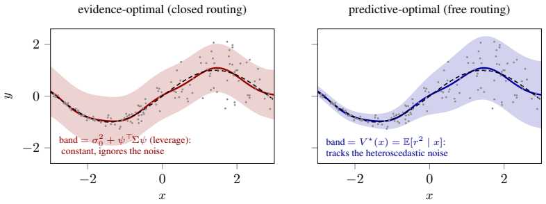
- [§4.1, Proposition 3 and Appendix C.2] The proof of Proposition 3 is incomplete at the load-bearing step. It shows that the free-route feasible set V_free = {σ_obs^2 + ψ_n^T Σ ψ_n : Σ ⪰ 0, σ_obs^2 ≥ 0} contains the closed-route profile, and therefore inf over V_free ≤ inf over V_closed. But the proposition claims that the free route 'represents' the predictive optimum V*(x) = E[(y−μ^Tψ)^2 | x]. Containing the closed route says nothing about whether V* lies in V_free. Since V_free is an affine image of the PSD cone of dimension at most 1+H(H+1)/2, for N exceeding this dimension a generic heteroscedastic V* is not representable by any PSD Σ. The paper's own data-rich regime (N ≫ H, e.g., Year with N=515k and H=100) is precisely where this obstruction is strongest. Moreover, the objective includes the prior term −log Z_w (Eq. 8), which depends on Σ and biases the variance away from V* at finite N. Thus the statements 'the free r
- [§3, Eq. (4) and the definition of F_SC] The manuscript defines the shared-cavity loss F_SC as a factor-wise sum of local log-partition functions, with the statement that 'belief-entropy corrections that couple the plates are dropped (they cancel exactly for deterministic factors, Appendix B).' This is not the Bethe free energy as usually defined, which contains explicit entropy terms. The cancellation is shown only for deterministic factors; for general factors the dropped terms do not cancel, and the relation between F_SC and the Bethe free energy is therefore unclear. Since the paper's title and framing present this as a Bethe free energy minimization, the authors need to state precisely what objective is being minimized, what approximation the entropy dropping introduces, and why minimizing this surrogate is justified beyond the Gaussian last-layer instantiation. As written, the framework is an ad-hoc proper-scoring objecti
- [§4.1, Proposition 3 vs. joint training in §5] Proposition 3 fixes the mean function μ^Tψ and then considers the variance. The experiments train μ, Σ, σ_obs, α, and the backbone jointly, so the learned mean changes with the variance. The paper acknowledges this in the RMSE discussion (Appendix F), but the central explanatory claim—that SCROLL's NLL/calibration gains over the exact corner are 'exactly the residual heteroscedasticity'—is not supported by a fixed-mean theorem when the mean is not fixed. The observed gains could be due to a different mean, a different effective prior, or the larger variance family, rather than to the mechanism in Proposition 3. A controlled experiment that isolates the variance effect (e.g., fixing the mean at the closed-route optimum and then fitting only Σ, σ_obs) would be needed to support the attribution made in Section 5(ii).
- [§5 and Table 2, headline count] The headline claim 'a fixed SCROLL variant is best-or-tied on 7/8' is based on fielding three fixed covariance variants and counting a win if at least one of them wins. The appendix provides per-variant counts (SCROLL-Full alone is 6/8), which is helpful, but the main text should be more careful: with three variants, the probability that at least one appears best by chance is inflated. The per-variant result should be moved into the main text or the claim should be rephrased. This does not affect the broader empirical conclusion but it does affect the precision of the central empirical summary.
minor comments (5)
- [§4.1, Eq. (11)] The notation V_n is used both for the per-plate predictive variance and, in the population statement of Proposition 3, for a function V(x). Please distinguish the empirical and population objects, and state whether V(x) is restricted to the parametric family σ_obs^2 + ψ(x)^T Σ ψ(x) throughout.
- [Figure 1 caption] The caption says 'shaded: ±2 predictive sd' but the text above describes a variance band. Please make the units consistent (standard deviation or variance).
- [Appendix D, Table 5 caption] The caption contains 'gd/elbo', which appears to be a typo for 'closed/ELBO'. Please fix.
- [Appendix C.2] In the proof of the closed-route limitation, the phrase 'the closed profiles form a two-parameter family of residual-independent leverage curves' is imprecise: the closed covariance depends on α and σ_obs, but also on the feature matrix Ψ, so the family is not simply two-dimensional in the space of variance profiles. Please rephrase.
- [Appendix A, validation criterion] SCROLL is selected by validation NLL while MAP-based baselines are selected by validation MSE. The paper reports an oracle comparison showing the criterion has little effect, which is good. Still, the sentence 'the criterion neither favours SCROLL nor systematically penalises the MSE-selected baselines' is stronger than what a median/mean difference of 0.09 nats establishes; please report the distribution or worst-case difference.
Circularity Check
No significant circularity: the proper-score properties are proved from Jensen/Gibbs; empirical wins are external; the main weakness is an unproven representability assertion in Prop. 3, which is a correctness gap, not a circularity.
full rationale
The paper's derivation chain is self-contained and non-circular. Propositions 1 and 2 are proved directly from Jensen's and Gibbs' inequalities (Appendix C.1), and Proposition 3 is a statement about optimization of the defined Gaussian log-loss (Eq. 11) and variance representability; it does not define its target in terms of its conclusion. The claim that free routing 'reaches that score's optimum' is a description of training on the stated objective, not a prediction extracted from fitted values. The empirical NLL/calibration comparisons are external benchmarks, not in-sample re-statements of the loss. No load-bearing self-citation occurs: the Bethe/BP/EP fixed-point facts are cited to Yedidia et al. and Minka, the neural-linear corner to Snoek/Ober/Rasmussen, and none of these citations is authored by the present paper or used to forbid alternatives. The main identified weakness—that the free-route variance family might not contain V*(x) for all x, so Prop. 3's representability step is asserted rather than proved—is a correctness/proof gap, not a circularity, and therefore does not raise the circularity score.
Assumptions & free parameters
free parameters (6)
- α (prior precision) =
learned by gradient descent (Eq. 8)
- σ_obs^2 (observation noise) =
learned (Eq. 11)
- Σ (last-layer covariance, V2/V3) =
learned (diag or LL^T with εI floor)
- μ (last-layer posterior mean) =
learned
- θ (backbone weights) =
learned
- ℓ2 penalty on backbone =
0.01
assumptions (5)
- ad hoc to paper The factor-wise sum F_SC in Eq. (4) is a valid Bethe/surrogate objective; dropped belief-entropy corrections cancel or are negligible.
- domain assumption Shared cavity β_n≈1 approximates the leave-one-out predictive when N≫H.
- domain assumption The predictive family can represent the true conditional p_true(y|x).
- ad hoc to paper V*(x)=E[(y-μ^Tψ)^2|x] is representable as σ_obs^2+ψ^TΣψ for a PSD Σ in the chosen family.
- domain assumption Data-rich regime N≫H holds on the benchmarks, so the selection gap is second-order.
Cite this review
Pith. "Pith review of Direct Bethe Free Energy Minimization for Bayesian Neural Networks." pith.science (2026). https://pith.science/paper/UPHINIGV
@misc{pith2026260508446,
  author       = {Pith},
  title        = {Pith review of: Direct Bethe Free Energy Minimization for Bayesian Neural Networks},
  year         = {2026},
  howpublished = {\url{https://pith.science/paper/UPHINIGV}},
  note         = {Machine review of arXiv:2605.08446}
}
read the original abstract
Bayesian neural networks are typically trained on the evidence lower bound (ELBO), which keeps the joint likelihood but pays a Jensen gap at every observation. We train by local consistency instead: direct minimisation of the Bethe free energy, whose data term pays no gap-it scores each observation exactly by its predictive density, a strictly proper rule, for any likelihood with a tractable predictive convolution. Our departure is free routing: the beliefs are trained as free parameters of this objective, jointly with the backbone, rather than bound to the conjugate posterior computed in closed form (closed routing). Instantiated with a Gaussian last layer over a deterministic backbone, exact inference appears as the known, closed-routed corner-the neural-linear marginal likelihood, evidence-optimal, keeping the joint. A shared cavity instead trades it for a batchable per-plate predictive score, and free routing reaches that score's optimum-unattainable under the binding whenever the noise is heteroscedastic-improving NLL and calibration over the exact corner. This instance, SCROLL (Shared-Cavity fRee-rOuting Last-Layer), is a single-pass, any-likelihood Bayesian neural network, implicitly empirical-Bayes-prior precision, observation noise, covariance, and backbone fit in one gradient pass. At a single training run and forward pass per architecture-where the conventional references cross-validate their regularisation weight and ensembles pay 5-50x at inference-a fixed SCROLL variant is best-or-tied on NLL and calibration on 7/8 UCI regression benchmarks, and best on 4/5 across three large tabular datasets and two frozen text/vision embeddings.
Figures


Figures from the paper (5 more)


Reference graph
Works this paper leans on
-
[2]
C.4 General Predictive Consistency Beyond Gaussian Proposition 2 states that the shared-cavity data term is a proper predictive score foranylikelihood— its population optimum is the true conditional—which is what makes the framework more than 16 102 103 training plates N 10 4 10 3 10 2 10 1 excess test NLL KL(true || model) (nats) Shared-cavity objective ...
2026
-
[3]
The UCI headline is full-batch; the large-scale runs sum the data term over a mini-batch
11 Algorithm 1SCROLL—Gaussian last-layer regression instance (Equation (11)). The UCI headline is full-batch; the large-scale runs sum the data term over a mini-batch. Require:data{(x n, yn)}; parametersθ(backbone),µ,Σ(belief),σ obs,α Training(all parameters in one gradient loop) 1:repeat 2:ψ n ←NN θ(xn)▷deterministic features 3:V n ←σ 2 obs +ψ ⊤ n Σψ n ▷...
-
[4]
each intermediate factor a is an activation transition p(hn,l |h n,l−1, wl). Adeterministiclayer with point-mass weight belief q(wl) =δ(w l −w ⋆ l )has fa(hn,l−1, hn,l) =δ hn,l −φ l(hn,l−1) , φ l(·) :=ϕ w⋆ l · ,(12) whereϕis the fixed elementwise nonlinearity and the affine map uses the point-mass weightw ⋆ l . Local partition function.The Bethe contribut...
2001
-
[5]
Predictive consistency (Proposition 2).By Gibbs’ inequality Ey∼p[−logm] =H(p) + KL(p∥m)≥ H(p), with equality iff m=p
Bethe–ELBO inequality (Proposition 1).By Jensen’s inequality on the concave logarithm, logZ n = logE q[p(yn |f n)]≥E q[logp(y n |f n)]; negating gives−logZ n ≤E q[−logp(y n |f n)]. Predictive consistency (Proposition 2).By Gibbs’ inequality Ey∼p[−logm] =H(p) + KL(p∥m)≥ H(p), with equality iff m=p . Applied per plate to the predictive mn(y) = R p(y|f)q(f n...
2022
-
[7]
The closed corner is best or statistically tied with the strongest baseline on all three modalities (text 0.88, vision 0.91, wine 0.95), beating its own free route by +0.21 to +0.31 AUROC. The free route—the headline’s NLL and calibration winner—is the weakest structured method here, and pays for the closed corner’s detection in reverse: the OOD gain cost...
-
[8]
evidence-optimal is not predictive-optimal
is also the better-calibrated one. Table 6: Regression calibration error, same validation-selected protocol and markup as the NLL table (Table 2, top block). yacht concrete energy kin8nm naval power wine boston SCROLL-Full0.0720.0440.0410.0150.2220.012 0.023 0.044 SCROLL-Diag0.0820.0460.049 0.0150.2110.011 0.022 0.037 SCROLL-None 0.1010.0320.050 0.0160.28...
-
[2001]
Joost van Amersfoort, Lewis Smith, Andrew Jesson, Oscar Key, and Yarin Gal. On feature collapse and deep kernel learning for single forward pass uncertainty.arXiv preprint arXiv:2102.11409,
-
[2016]
Richer Bayesian last layers with subsampled NTK features
Sergio Calvo-Ordóñez, Jonathan Plenk, Richard Bergna, Álvaro Cartea, Yarin Gal, José Miguel Hernández-Lobato, and Kamil Ciosek. Richer Bayesian last layers with subsampled NTK features. arXiv preprint arXiv:2602.01279,
Reviewed August 2, 2026 · model on record in the stance chip above.
Discussion (0). Continue with ORCID to comment.