REVIEW 2 major objections 4 minor 83 references
Diffusion equation and rare fluctuations of the biased aging continuous-time random walk model
T0 review · 2 major / 4 minor · reviewed 2026-08-12 · deepseek-v4-flash
Pith's one-line read Biased aging random walks with fat-tailed waiting times are shown to obey a fractional advection-diffusion equation in space, with an aging-dependent infinite-density tail describing their rare fluctuations.
desk verdict New finite-aging-time results, essentially correct; the main gap is a heuristic two-scale step that should be stated as an asymptotic ordering, not a fatal flaw. read the letter →
The pith
A machine-rendered reading of the paper's core claim, the machinery that carries it, and where it could break.
The reading
What carries the argument
The load-bearing object is the subordination formula $P(x,t_a,t)=\sum_N Q_{t_a,t}(N)f(x|N)$, combined with the double-Laplace renewal representation of $Q_{t_a,t}(N)$. In the long-time, small-$k$ limit the key move is to neglect the Gaussian width term $\sigma^2 k^2$ inside the Levy-stable factor while keeping it in the advection-diffusion factor; this converts the stable factor into $\exp[(-ika)^\alpha y/\bar t]$ and produces the fractional space derivative. The second structural object is the dimensionless variable $\zeta=1-(x/a)/(t/\langle\tau\rangle)$, which isolates the rare-event region where $x-at/\langle\tau\rangle$ is of order $t$ and turns the tail into the explicit infinite-density forms.
What would settle it
Numerically invert the unsimplified Fourier expression (18) with the $\sigma^2 k^2$ term retained in the Levy-stable factor, and compare the result with Eq. (19) for $\alpha=3/2$, $\tau_0=0.1$, $t=t_a=1000$, $a=1$, $\sigma=1$; if the difference does not vanish as $t$ grows, the central fractional equation fails. Independently, the paper's own statement that Eq. (21) yields an infinite second moment can be checked against simulated MSD from the rare-event tail: if the MSD predicted by Eq. (31) deviates from simulations at finite $t_a$, the tail claim is falsified.
Extended reading notes
Core claim
In the paper's own terms, the central discovery is that the long-time position PDF of the biased ACTRW with $1<\alpha<2$ solves $$\frac{\partial P}{\partial t}=D\frac{\$partial^{2}$ P}{\partial $x^{2}$}-V\frac{\partial P}{\partial x}+S\frac{\partial^\$\alpha$ P}{\partial(-x)^\$\alpha$}+\omega(t_a,t)\delta(x),$$ with $D=\sigma^2/(2\langle\tau\rangle)$, $V=a/\langle\tau\rangle$, $S=a^\alpha/\bar t$, and with a right Riemann-Liouville fractional derivative in space. The far tail is the infinite density $$P(x,t_a,t)\sim\frac{\tau_0^\$\alpha$}{a t^\$\alpha$\$zeta^{{1+\alpha}}$}\bigl[\$\alpha$+(2-\$\alpha$)\zeta\bigr]-\frac{\tau_0^\$\alpha$}{a t^\$\alpha$}\left(\zeta+\frac{t_a}{t}\right)^{-\$\alpha$}+\frac{\tau_0^\$\alpha$}{\langle\tau\rangle(1-\$\alpha$)}\bigl[(t+t_a)^{1-\$\alpha$}-$t^{{1-\alpha}}$\bigr]\delta(x),$$ where $\zeta=1-(x/a)/(t/\langle\tau\rangle)$. The tail is non-integrable, depends on $t_a$ through the ratio $t_a/t$, and controls the mean-squared displacement, whereas the central part of the distribution is aging-insensitive. The same method gives the far tail of the number of renewals, $$Q_{t_a,t}(\epsilon)\sim\tau_0^\$\alpha$\left[\frac{2-\$\alpha$}{(-\langle\tau\rangle\epsilon)^\$\alpha$}+\frac{\$\alpha$ t}{(-\langle\tau\rangle\epsilon)^{1+\$\alpha$}}\right]-\frac{\tau_0^\$\alpha$}{(t_a-\langle\tau\rangle\epsilon)^\$\alpha$},$$ tying position and renewal rare events through $x\sim aN$.
Load-bearing premise
The derivation assumes that, at long times, the finite width of the jump lengths stops mattering inside the fractional part of the equation even though it still sets the ordinary diffusion constant; this two-scale split is the load-bearing approximation and is not derived from a controlled expansion.
Editorial extensions
If this is right
- The fractional operator in the kinetic equation is spatial even though the jump distribution is Gaussian: a fat-tailed waiting time plus a bias is sufficient, so power-law jumps are not required for fractional space transport.
- Typical fluctuations of position follow the same aging-insensitive Levy stable form, while the far tail depends on $t_a/t$; therefore tail measurements can estimate the aging time even when the central part cannot.
- The mean displacement is linear, with speed $a/\langle\tau\rangle$, but the second moment is infinite under the fractional equation; the MSD must be computed from the rare-event tail, which gives a $t^{3-\alpha}$-type growth with $t_a$-dependent corrections.
- The far tail of position and the far tail of the number of renewals are governed by the same rare-event mechanism through $x\sim aN$, so observing one tail predicts the other.
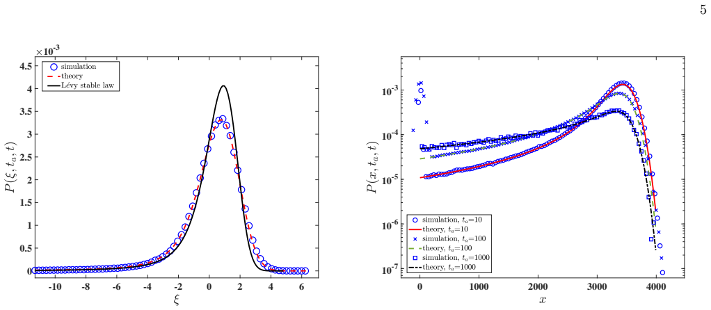
- The aging fractional equation also covers the modified ACTRW with different power-law indices before and after the observation start, which is confirmed by simulation.
Reading between the lines
- A testable consequence the authors leave implicit: for any narrow displacement distribution with finite nonzero mean and variance, not just Gaussian, the same two-scale approximation should yield Eq. (21) with the same $D$, $V$, $S$; a simulation with Laplace or asymmetric jump distributions would check whether the constants remain universal.
- The two-scale approximation predicts a crossover: when $\sigma$ is large or $a$ is small, the neglected $\sigma^2 k^2$ term in the stable factor may matter at intermediate times; measuring the convergence rate of the central part to the Levy-stable form would quantify when the fractional equation becomes valid.
- The delta-source term in Eq. (21) means non-moving particles contribute mass at the origin; a natural extension is the full time-dependent solution for all $t_a$, which would interpolate between the CTRW and equilibrium limits and could be compared with the infinite-density tail at finite $t_a$.
- Because the tail is an infinite density, its normalization is not defined; this suggests that any coarse-grained binning in simulations must be handled with care, and that integrated tail probabilities rather than pointwise PDF values are the more robust observable for comparing theory and experiment.
Signed reviews
Editorial analysis
A structured set of objections, weighed in public.
Referee Report
Summary. The paper studies the biased aging continuous-time random walk (ACTRW) with power-law waiting times of index 1<α<2 (finite mean, infinite variance) and Gaussian displacements with mean a and variance σ². Using the subordination representation and double Laplace/Fourier transforms, it derives an aging fractional advection-diffusion equation (Eq. (21)) with advection and diffusion constants V=a/⟨τ⟩, D=σ²/(2⟨τ⟩), a spatial fractional derivative with strength S=a^α/t̄, and an aging-dependent source term. It further derives the far tail of the position distribution in the form of an infinite density (Eq. (31)), the corresponding asymptotic MSD (Eq. (40)), and analogous far-tail results for the renewal count (Eqs. (45), (47), (50)). The analytical predictions are compared with simulations for several aging times and for a modified ACTRW with different α in the preparation interval.
Significance. If the asymptotic ordering is made explicit, the paper is a useful contribution. It shows that a fractional space operator can arise from heavy-tailed waiting times rather than heavy-tailed jumps, gives explicit parameter-free transport constants, demonstrates that typical fluctuations are largely aging-insensitive while rare fluctuations are not, and recovers the known limits ta→0 and ta→∞ of [13] and the equilibrium CTRW. The simulation checks use large sample sizes and cover several aging times, and the constants in Eqs. (22), (31), and (45) are expressed in terms of model inputs with no fitted parameters. The main weakness is that the key step from Eq. (18) to Eq. (19) rests on an unstated smallness condition; this is a load-bearing point that needs to be clarified before the central equation can be considered established.
major comments (2)
- [Section III, Eq. (18) to Eq. (19)] The one-sentence justification for dropping (σ²/2)k² in the inner Lévy-stable factor is not a controlled asymptotic statement, and it is load-bearing for Eq. (21). With the Gaussian variance retained, the inner integral in Eq. (18) is exactly exp{[-ika − σ²k²/2]^α y/t̄} (up to the Fourier convention); passing to Eq. (19) replaces this by exp{(-ika)^α y/t̄}, discarding a correction of relative order α σ² k/a in the exponent. At the natural central scale k ∼ (t/t̄)^{-1/α} this correction is O((σ²/a)(t/t̄)^{-1/α}), which is small only under an ordering such as σ²/a ≪ (t/t̄)^{1/α}. This ordering is nowhere stated, and the same σ² is retained in the Gaussian factor exp(-σ²k²y/(2⟨τ⟩)) in the first line of Eq. (19), so the treatment is asymmetric. The simulations use a=0.5 or 1 with σ=1 at t=1000, for which the omitted correction is only a few percent; they do not probe regimes where a is small or σ is large. Please state the required ordering and justify the two-scale separation, or reformulate Eq. (21) as a leading-order approximation with an explicit error estimate.
- [Section V, Eq. (45)] The domain of validity of Eq. (45) is not stated precisely enough. The derivation assumes s + ik/⟨τ⟩, u, and s are all small and comparable, which corresponds to ε = N − t/⟨τ⟩ of order t. As written, Eq. (45) is asserted for 'both ta and t are large' without restricting ε. For |ε| ≫ t, the first and third terms in Eq. (45) cancel at leading order, leaving a term proportional to (1−α)/(−⟨τ⟩ε)^α, which is negative for 1<α<2; hence the formula becomes non-positive in the far tail. The paper should explicitly state that Eq. (45) applies in the scaling region ε = O(t), and should not be interpreted as an arbitrarily deep tail.
minor comments (4)
- [Eq. (23)] In Eq. (23), the stable-density normalization appears to contain an extra factor 1/α after (1/(t/t̄)^{1/α}); this should be removed so that the convolution kernel is the normalized stable density.
- [Section III, Eq. (24)] The phrase 'Clearly, this prediction is wrong' is too strong: the fractional equation is intended to describe typical fluctuations, and its divergent second moment indicates that moments are not captured by this bulk description rather than that the equation is false. Please rephrase to avoid implying that Eq. (21) is invalidated by this property.
- [General] There are numerous minor typographical errors, such as 'obtained' in the introduction, missing articles in several figure captions, and the caption of Fig. 1 reading 'Comparison Eq. (21) with...' instead of 'Comparison of Eq. (21) with...'. A careful proofread is advised.
- [Section IV, Eq. (31)] The delta-function contribution in Eq. (31) is written with a coefficient that is positive for 1<α<2 (after combining the two negatives), but this is not obvious from the displayed formula; a brief explanation of the origin and sign of the non-moving-particle term would improve readability.
Circularity Check
No circularity found: the derivation is self-contained, with all transport constants expressed through model inputs and no fitted parameter renamed as a prediction.
full rationale
I traced the main derivation chain from the subordination formula Eq. (7) and the renewal representation Eq. (8) to the Fourier-space expression Eq. (19) and the fractional advection-diffusion equation Eq. (21). The passage from Eq. (18) to Eq. (19) is a stated asymptotic approximation (dropping sigma^2 k^2/2 in the stable factor for k to 0); whether the ordering is justified is a correctness question, not a circular one, because the target equation is not used to justify the step. The coefficients in Eq. (22) are expressed directly in the model parameters (D=sigma^2/(2<tau>), V=a/<tau>, S=a^alpha/tbar), so no fitted parameter is renamed as a prediction. The far-tail result Eq. (31) follows from Laplace-space expansions of the generalized Montroll-Weiss equation Eq. (25), with the ta to 0 and ta to infinity limits matching the earlier published results [13] only as consistency checks; Eq. (45) for the renewal tail is derived separately from Eq. (42), not obtained by simply renaming Eq. (31). Simulations are external validations throughout. Self-citations [13,19,25] supply background, the double-Laplace first-waiting-time form Eq. (1), and limiting forms; none of them carries a load-bearing uniqueness claim or injects the advertised result as an assumption. I therefore find no step in which an output is equivalent to an input by construction.
Assumptions & free parameters
assumptions (7)
- domain assumption Renewal process with IID waiting times and the subordination formula P = sum_N Q(N) f(x|N) (Eq. 7) correctly describes the ACTRW.
- standard math The Laplace expansion of the waiting-time PDF, phi(s) ~ 1 - <tau>s + b_alpha s^alpha for s->0 (Eq. 4), is valid for 1<alpha<2.
- standard math The displacement characteristic function is expanded to order k^2 as f(k) ~ 1 + ika - (sigma^2+a^2)k^2/2 (Eq. 6), and higher orders are negligible in the long-time limit.
- domain assumption For large N, the double-Laplace renewal count factorizes as Q(u,s,N) ~ omega(u,s) Q(s,N) (Eq. 9).
- ad hoc to paper In the long-time limit, the term (1/2)sigma^2 k^2 inside the Levy-stable part of Eq. (18) can be neglected (Eq. 18 to 19).
- domain assumption The far tail of the position can be treated as an infinite density, i.e., a non-normalizable function that yields finite moments when integrated with appropriate cutoffs (Eq. 31).
- standard math The number of renewals N can be treated as a continuous variable in the Laplace representation (Eqs. 41-42).
Cite this review
Pith. "Pith review of Diffusion equation and rare fluctuations of the biased aging continuous-time random walk model." pith.science (2026). https://pith.science/paper/VGL6EDHR
@misc{pith2026241109989,
  author       = {Pith},
  title        = {Pith review of: Diffusion equation and rare fluctuations of the biased aging continuous-time random walk model},
  year         = {2026},
  howpublished = {\url{https://pith.science/paper/VGL6EDHR}},
  note         = {Machine review of arXiv:2411.09989}
}
read the original abstract
We explore the fractional advection-diffusion equation and rare events associated with the ACTRW model. When waiting times have a finite mean but infinite variance, and the displacements follow a narrow distribution, the fractional operator is defined in terms of space rather than time. The far tail of the positional distribution is governed by rare events, which exhibit a different scaling compared to typical fluctuations. Additionally, we establish a strong relationship between the number of renewals and the positional distribution in the context of large deviations. Throughout the manuscript, the theoretical results are validated through simulations.
Figures


Figures from the paper (4 more)


Reference graph
Works this paper leans on
-
[13]
to high- light the relationship between the CTR W model and the equilibrium CTR W model, specifically for ta ≪ t and t ≪ ta, which correspond to weakly aging and strongly aging systems, respectively. The key idea, based on Eq. ( 27), is to calculate the following term ˆh(u) u − s = 1 u − s 1 1 −ˆφ(u) ∼ 1 u − s 1 ⟨τ ⟩u − bα uα . (32) When both s and u are s...
-
[25]
The inverse Fourier-Laplace transform is straightforward for this term
corresponds to the case where the num- ber of renewals is zero, describing non-moving particles. The inverse Fourier-Laplace transform is straightforward for this term. Below, we focus on the moving term in Eq. ( 25). Unlike Eq. ( 21), we consider the scaling when x − at/⟨τ ⟩ is of the order of t. Substituting Eq. ( 1) into the second term of Eq. ( 25), w...
-
[1]
Metzler and J
R. Metzler and J. Klafter, Phys. Rep. 339, 1 (2000)
2000
-
[2]
J. Klafter and I. M. Sokolov, First Steps in Random Walks: From Tools to Applications (Oxford University Press, Oxford, 2011)
work page 2011
-
[3]
but with an infinite mean, i.e., 0 < α = α1 < 1, while in the time interval (0, t), waiting times are drawn from Eq. ( 3) with 1 < α = α2 < 2. All along the process, the displacements are drawn from Eq. ( 5). Figure 3 indicates that Eq. ( 21) provides an accurate prediction. Using the relationship between the characteristic func- tion and moments, Eq. ( 19...
-
[4]
follows P(x, ta, t) =ω(ta, t) ⊗t [ ( 1 (t/¯t) 1 α ) 1 α Lα ( x (t/¯t) 1 α ) ⊗x exp ( − (⟨τ ⟩x−at)2 2t⟨τ ⟩σ 2 ) √ 2πσ2t/⟨τ ⟩ , (23) where ⊗t and ⊗x are the convolution of t and x, respec- tively. In Fig. 1, Eq. ( 23) is compared with the asym- metric L´ evy stable law, showing an excellent agreement with the simulations. In our comparison, we find that Eq. (
-
[5]
P. P¨ oschke, I. M. Sokolov, A. A. Nepomnyashchy, and M. A. Zaks, Phys. Rev. E 94, 032128 (2016)
work page 2016
-
[6]
Notably, N is expected to exhibit a cutoff at the tail N = 0. It can be seen that the strong relation between the position and the number of renewals is x ∼ aN ∼ at/⟨τ ⟩ obtained using large deviations. Similarly to the discussion of the position, we further explore the limits of Eq. ( 45), specifically for the cases ta ≪ t and t ≪ ta. These two limits aris...
Show all 83 references
-
[7]
and ( 11), we obtain P (x, ta, t) ∼ ∫ ∞ 0 exp ( − (x−aN )2 2σ 2N ) √ 2πσ2N × ∫ t 0 ω(ta, t − y) (y/¯t)1/α Lα (N − y/⟨τ ⟩ (y/¯t)1/α ) dydN, (14) where we have used the fact that displacements are IID random variables drawn from Eq. ( 5). Changing the vari- ables ξ = ( N − y/⟨τ ...
-
[8]
( 21) are infinite
fails, as the second mo- ments of the positions obtained from Eq. ( 21) are infinite. Clearly, this prediction is wrong. Besides, when the ob- servation time is long, and the bias is strong, there is no big gap for different aging times in the context of the central part of the ...
-
[9]
( 13) describing typical fluctuations of the position
and the L´ evy stable law shows typical fluctuations of the positi on obtained from Eq. ( 13) describing typical fluctuations of the position. We use the parameters α = 3/2, τ0 = 0.1, t = 1000, ta = 1000, a = 1/2, and σ = 1. 0 500 1000 1500 2000 2500 3000 3500 4000 10-1 100 101 ...
2000
-
[10]
and the solid line obtained from Eq. ( 13). We use the parameters α = 3/2, τ0 = 0.1, t = 1000, ta = 1000, a = 1, and σ = 1. IV. RARE EVENTS OF THE POSITION In this section, we focus on large deviations of the po- sition distribution, specifically analyzing the scaling be- havio...
2000
-
[11]
(25) Equation ( 25) is a generalized Montroll Weiss equation describing ACTR W
and ( 8), the positional distribution ~ˆP (k, u, s) in Fourier-Laplace spaces is given by [ 7, 35] ~ˆP (k, u, s) = 1 −ˆω(u, s) s + 1 −ˆφ(s) s ~f (k)ˆω(u, s) 1 − ~f (k)ˆφ(s) . (25) Equation ( 25) is a generalized Montroll Weiss equation describing ACTR W. The first term on the r...
-
[12]
When the aging time ta tends to infinity and the ob- servation time t is long, the positional distribution con- verges to the well-known L´ evy stable law, as derived us- ing Eqs
demon- strates an asymmetric behavior of N characterized by a fat tail and a narrow one. When the aging time ta tends to infinity and the ob- servation time t is long, the positional distribution con- verges to the well-known L´ evy stable law, as derived us- ing Eqs. ( 4), ( 6...
-
[14]
R. Hou, A. G. Cherstvy, R. Metzler, and T. Akimoto, Phys. Chem. Chem. Phys. 20, 20827 (2018)
2018
-
[15]
Magdziarz and T
M. Magdziarz and T. Zorawik, Phys. Rev. E 95, 022126 (2017)
2017
-
[16]
(41) Given our interest in the long-time behavior, where N can be treated as a continuous variable, performing the integral over N in Eq
and applying the Laplace trans- form with respect to N , we obtain ˆQta,s (v) ∼ˆω(ta, s) 1 −ˆφ(s) s × ∫ ∞ 0 exp{−vN + N ln[ˆφ(s)]}dN. (41) Given our interest in the long-time behavior, where N can be treated as a continuous variable, performing the integral over N in Eq. (
-
[17]
Allegrini, G
P. Allegrini, G. Aquino, P. Grigolini, L. Palatella, A. Rosa, and B. J. West, Phys. Rev. E 71, 066109 (2005)
2005
-
[18]
B. J. West, E. L. Geneston, and P. Grigolini, Phys. Rep. 468, 1 (2008). 12
2008
-
[19]
W. Wang, J. H. P. Schulz, W. H. Deng, and E. Barkai, Phys. Rev. E 98, 042139 (2018)
2018
-
[20]
For instance, when waiting times have an infinite mean, the generalized master equation serves as a framework that unifies fractional calculus with CTR W
The diffusion equation for random walks can also be derived from the generalized master equation [ 8, 9]. For instance, when waiting times have an infinite mean, the generalized master equation serves as a framework that unifies fractional calculus with CTR W. However, the approa...
-
[21]
Furthermore, Eq
reduces to the fractional advection- diffusion asymmetric equation for the CTR W model [ 25]. Furthermore, Eq. ( 21) indicates that a fat tail of the dis- placement distribution is not necessary for the emergence of a fractional space operator, as discussed in [ 25]. The method...
-
[22]
and the number of renewals in Eq. ( 45). As expected, our results align with those in [ 13] when considering the limits ta → 0 or ta → ∞. It is important to note that the rare events of renewals discussed in this manuscript differ from those in [ 30, 61], which focus on the sho...
-
[23]
2 when the time is long and the bias is strong
is not sensitive to the aging time ta as shown in Fig. 2 when the time is long and the bias is strong. To further validate Eq. ( 21), we consider a more mathematically complex model, i.e., a modified ACTR W model. In this model, during the time interval ( −ta, 0), waiting times...
-
[24]
Appendix C: MOMENTS OF THE POSITION obtained from rare fluctuations Now, we show the derivation process of the MSD for ACTR W using rare fluctuations
in the main text. Appendix C: MOMENTS OF THE POSITION obtained from rare fluctuations Now, we show the derivation process of the MSD for ACTR W using rare fluctuations. Based on Eq. ( 31), we have 11 ⟨( x − at ⟨τ ⟩ ) 2⟩ = ∫ ∞ −∞ ( x − at ⟨τ ⟩ ) 2 P (x, ta, t)dx ∼ (at)2 ⟨τ ⟩2 τ α...
-
[26]
Brokmann, J.-P
X. Brokmann, J.-P. Hermier, G. Messin, P. Desbiolles, J.-P. Bouchaud, and M. Dahan, Phys. Rev. Lett. 90, 120601 (2003)
2003
-
[27]
A. V. Weigel, B. Simon, M. M. Tamkun, and D. Krapf, PNAS 108, 6438—6443 (2011)
2011
-
[28]
M. S. Song, H. C. Moon, J.-H. Jeon, and H. Y. Park, Nat. Commun. 9, 344 (2018)
2018
-
[29]
Barkai, Phys
E. Barkai, Phys. Rev. Lett. 90, 104101 (2003)
2003
-
[30]
Metzler, Phys
R. Metzler, Phys. Rev. E 62, 6233 (2000)
2000
-
[31]
As shown in Fig
is called an infinite density [ 60]. As shown in Fig. 4, the far tail of the positional distribution becomes sensitive to the aging time of the systems and is well described by Eq. ( 31). This is because the MSD is highly influenced by the slow-moving particles that lag significa...
-
[32]
Allegrini, G
P. Allegrini, G. Aquino, P. Grigolini, L. Palatella, and A. Rosa, Phys. Rev. E 68, 056123 (2003)
2003
-
[33]
J. H. P. Schulz, E. Barkai, and R. Metzler, Phys. Rev. Lett. 110, 020602 (2013)
2013
-
[34]
Busani, Electronic Journal of Probability 21 (2016)
O. Busani, Electronic Journal of Probability 21 (2016)
2016
-
[35]
J. H. P. Schulz, E. Barkai, and R. Metzler, Phys. Rev. X 4, 011028 (2014)
2014
-
[36]
W. Wang, A. Vezzani, R. Burioni, and E. Barkai, Phys. Rev. Res. 1, 033172 (2019)
2019
-
[37]
Taking ta → ∞ , Eq
is determined by the aging time ta and the observation time t. Taking ta → ∞ , Eq. (37) aligns with the theory for the equilibrium CTR W model discussed in [ 13], since the second term disappears. Using the far tail of the position provided in Eq. ( 30), the MSD of the positio...
-
[38]
Allegrini, P
P. Allegrini, P. Grigolini, L. Palatella, and B. J. West , Phys. Rev. E 70, 046118 (2004)
2004
-
[39]
Aquino, M
G. Aquino, M. Bologna, B. J. West, and P. Grigolini, Phys. Rev. E 83, 051130 (2011)
2011
-
[40]
0 0.5 1 10-1 100 102 ordinary process equilibrium process theory simulation 0.6 0.8 1 0.05 0.15 0.25 FIG
can also be derived using the relationship be- tween the moments and the characteristic function. 0 0.5 1 10-1 100 102 ordinary process equilibrium process theory simulation 0.6 0.8 1 0.05 0.15 0.25 FIG. 5: The Scaled PDF when ta ≪ t, where ζ = 1 − (x/a)/(t/⟨τ ⟩). The solid li...
-
[41]
(42) To further analyze the system, we introduce the new ran- dom variable ǫ = N − t/⟨τ ⟩ and investigate its statistics
yields ˆQta,s (v) ∼ˆω(ta, s) 1 −ˆφ(s) s 1 v − ln(ˆφ(s)) . (42) To further analyze the system, we introduce the new ran- dom variable ǫ = N − t/⟨τ ⟩ and investigate its statistics. After performing the Fourier transform with respect to ǫ (i.e., ǫ → k) and the double Laplace tra...
-
[42]
(43) Mathematically, the solution of Qta,t (N ) can be approxi- mated by Eq
in Fourier-Laplace spaces, is given by 8 ˆQu,s (k) ∼ ˆφ(s + ik ⟨τ ⟩) −ˆφ(u) (u − s − ik ⟨τ ⟩)(1 −ˆφ(u)) 1 −ˆφ(s + ik ⟨τ ⟩) s + ik ⟨τ ⟩ × 1 −ik − ln(ˆφ(s + ik ⟨τ ⟩)) . (43) Mathematically, the solution of Qta,t (N ) can be approxi- mated by Eq. ( 11), with Qt(N ) following the ...
-
[43]
Metzler, E
R. Metzler, E. Barkai, and J. Klafter, Phys. Rev. Lett. 82, 3563 (1999)
1999
-
[44]
Barkai, Phys
E. Barkai, Phys. Rev. E 63, 046118 (2001)
2001
-
[45]
Magdziarz, A
M. Magdziarz, A. Weron, and J. Klafter, Phys. Rev. Lett. 101, 210601 (2008)
2008
-
[46]
Deng, SIAM J
W. Deng, SIAM J. Numer. Anal. 47, 204 (2009)
2009
-
[47]
A. V. Chechkin, R. Gorenflo, and I. M. Sokolov, J. Phys. A: Math. Gen. 38, L679 (2005)
2005
-
[48]
Wang and E
W. Wang and E. Barkai, Phys. Rev. Lett. 125, 240606 (2020)
2020
-
[49]
Wang and E
W. Wang and E. Barkai, J. Phys. A: Math. Theor. 57, 035203 (2024)
2024
-
[50]
Metzler, E
R. Metzler, E. Barkai, and J. Klafter, EPL 46, 431 (1999)
1999
-
[51]
Metzler, J
R. Metzler, J. Klafter, and I. M. Sokolov, Phys. Rev. E 58, 1621 (1998)
1998
-
[52]
Chaudhuri, L
P. Chaudhuri, L. Berthier, and W. Kob, Phys. Rev. Lett. 99, 060604 (2007)
2007
-
[53]
Barkai and S
E. Barkai and S. Burov, Phys. Rev. Lett. 124, 060603 (2020)
2020
-
[54]
W. Wang, E. Barkai, and S. Burov, Entropy 22, 697 (2020)
2020
-
[55]
Burov, W
S. Burov, W. Wang, and E. Barkai, Exponential tails and asymmetry relations for the spread of biased random walks. ArXiv:2209.03410
-
[56]
Vezzani, E
A. Vezzani, E. Barkai, and R. Burioni, Phys. Rev. E 100, 012108 (2019)
2019
-
[57]
Monthus and J.-P
C. Monthus and J.-P. Bouchaud, J. Phys. A: Math Theor. 29, 3847 (1996)
1996
-
[58]
Barkai and Y
E. Barkai and Y. C. Cheng, J. Chem. Phys. 118, 6167 (2003)
2003
-
[59]
W. L. Wang and W. H. Deng, J. Phys. A 51, 015001 (2018)
2018
-
[60]
Godr` eche and J
C. Godr` eche and J. M. Luck, J. Stat. Phys. 104, 489 (2001)
2001
-
[61]
Aquino, M
G. Aquino, M. Bologna, P. Grigolini, and B. J. West, Phys. Rev. Lett. 105, 040601 (2010)
2010
-
[62]
Levy and B
M. Levy and B. Berkowitz, J. Contam. Hydrol. 64, 203 (2003)
2003
-
[63]
Burioni, G
R. Burioni, G. Gradenigo, A. Sarracino, A. Vezzani, and A. Vulpiani, J. Stat. Mech. Theory Exp. 2013, P09022 (2013)
2013
-
[64]
Nissan, I
A. Nissan, I. Dror, and B. Berkowitz, Water Resour. Res. 53, 3760 (2017)
2017
-
[65]
W. Deng, R. Hou, W. Wang, and P. Xu, Modeling Anomalous Diffusion: From Statistics to Mathematics (World Scientific, Singapore, 2020)
2020
-
[66]
T. Zhou, P. Xu, and W. Deng, Phys. Rev. Res. 2, 013103 (2020)
2020
-
[67]
A. S. Bodrova and I. M. Sokolov, Phys. Rev. E 101, 062117 (2020)
2020
-
[68]
J. Liu, Y. Hu, and J.-D. Bao, J. Stat. Mech: Theory Exp. 2023, 073202 (2023)
2023
-
[69]
Margolin and B
G. Margolin and B. Berkowitz, Phys. Rev. E 65, 031101 (2002)
2002
-
[70]
C. F. E. Schroer and A. Heuer, Phys. Rev. Lett. 110, 067801 (2013)
2013
-
[71]
Luo and L.-H
L. Luo and L.-H. Tang, Phys. Rev. E 92, 042137 (2015)
2015
-
[72]
X. Wang, Y. Chen, and W. Deng, Phys. Rev. Res. 2, 013102 (2020)
2020
-
[73]
Zhang, Y
C. Zhang, Y. Hu, and J. Liu, J. Stat. Mech: Theory Exp. 2022, 093205 (2022)
2022
-
[74]
Bouchaud and A
J.-P. Bouchaud and A. Georges, Phys. Rep. 195, 127 (1990)
1990
-
[75]
Klafter and G
J. Klafter and G. Zumofen, J. Phys. Chem. 98, 7366 (1994)
1994
-
[76]
Sandev and A
T. Sandev and A. Iomin, Phys. Rev. E 110, 024101 (2024)
2024
-
[77]
Semeraro, Mathematics and Financial Economics 16, 685 (2022)
P. Semeraro, Mathematics and Financial Economics 16, 685 (2022)
2022
-
[78]
K. B. Oldham and J. Spanier, The Fractional Calculus (Academic Press, New York, 1974)
1974
-
[79]
D. A. Benson, S. W. Wheatcraft, and M. M. Meerschaert, Water Resour. Res. 36, 1413 (2000)
2000
-
[80]
Podlubny, Fractional Differential Equations (Academic Press, Inc., San Diego, 1999)
I. Podlubny, Fractional Differential Equations (Academic Press, Inc., San Diego, 1999)
1999
-
[81]
W. H. Deng and Z. J. Zhang, High Accuracy Algorithm for the Differential Equations Governing Anomalous Dif- fusion: Algorithm and Models for Anomalous Diffusion (World Scientific, Singapore, 2018)
2018
-
[82]
Rebenshtok, S
A. Rebenshtok, S. Denisov, P. H¨ anggi, and E. Barkai, Phys. Rev. E 90, 062135 (2014)
2014
-
[83]
Wang and S
W. Wang and S. Burov, Statistics of a large number of renewals in equilibrium and non-equilibrium renewal pro- cesses (2024)
2024
Reviewed August 12, 2026 · model on record in the stance chip above.
Discussion (0). Continue with ORCID to comment.