REVIEW 4 major objections 6 minor 33 references
Continual Learning via Ensemble-Based Depth-Wise Masked Autoencoders for Data Quality Monitoring in High-Energy Physics
T0 review · 4 major / 6 minor · reviewed 2026-08-02 · deepseek-v4-flash
Pith's one-line read This paper claims that a lightweight, continually refreshed ensemble of depth-wise masked autoencoders keeps anomaly-detection precision above 98.8% on CMS detector data even as the data distribution shifts between 2018 and 2022, without th
desk verdict Useful controlled study of a lightweight continual-learning DQM system, but the pristine-data recalibration assumption is load-bearing and the evaluation is narrower than the abstract implies. read the letter →
The pith
A machine-rendered reading of the paper's core claim, the machinery that carries it, and where it could break.
The reading
What carries the argument
DepthViT (depth-wise masked autoencoder): a vision-transformer-style autoencoder whose patch embedding uses depth-wise convolution (each input channel gets its own filters, rather than summing over channels) and whose self-attention computes attention weights along the channel/depth axis instead of the spatial sequence axis. It is paired with a masked-reconstruction training objective and a latent-space variational resampling. The continual learning machinery is an ensemble of four such models, each trained on a different recent run and each applied to max-scaled and quantile-scaled inputs; an LS is flagged anomalous if any member's gap-score (the gap between the largest and second-largest p
What would settle it
Inject a known synthetic anomaly into the validation data used to recompute mu_err and sigma_err for a given run, then run the ensemble on that run's test data; if the injected anomaly is never flagged (recall near zero for that pattern), the pristine-data assumption would be falsified. A second test: replace the synthetic single-pixel multiplicative anomalies with a real detector fault signature (e.g., the 2018 dead region in a 40-degree azimuthal sector) and check whether the ensemble detects it as a single entity.
Extended reading notes
Core claim
DepthViT is a masked autoencoder with depth-wise convolutional patch embeddings and depth-wise attention, meaning each of the seven HCAL depth channels keeps its own kernels and attention is computed along the channel axis rather than the spatial patch axis. The authors report that on a single 2018 run a DepthViT sub-ensemble detects injected single-pixel anomalies with perfect precision and recall for most anomaly factors, but that the same static model degrades severely on later runs, reaching false-negative rates of 0.45–0.75 on 2022 data. Their continual learning method refreshes the per-pixel error statistics (mu_err, sigma_err) used in the Z-score baseline using each run's validation d
Load-bearing premise
The method relies on each new run providing a segment of 'pristine' (anomaly-free) data to recompute error statistics and train new ensemble members; if anomalies are present in that calibration data, they become part of the baseline and escape detection.
Editorial extensions
If this is right
- Detector quality monitoring can stay accurate over multi-year campaigns by retraining only on recent runs and keeping a small ensemble, rather than retraining on all historical data.
- The same continual learning recipe should apply to any monitoring setting where sensor readings drift with time, such as manufacturing lines or environmental sensors.
- Because DepthViT uses about 300k parameters, ensembling many models adds little computational cost; the paper notes the OR-ensemble is trivially parallelizable.
- The combination of refreshed statistics and ensembling specifically reduces false-negative rates (from 0.45–0.75 down to near zero for strong anomalies) while keeping false positives low (FPR 0.012).
Reading between the lines
- The evaluation uses synthetic single-pixel multiplicative anomalies; a natural next test is whether the ensemble detects extended, correlated real faults such as the 2018 dead azimuthal sector, which may behave differently under max and quantile scaling.
- The method requires a clean stretch of data for every run to refresh statistics; in practice, an online deployment might need a separate robust estimator of baseline statistics or a human-in-the-loop confirmation that the calibration window is anomaly-free.
- Depth-wise attention trades away spatial mixing between patches within a layer; this design could generalize to other multi-channel data where channels are not aligned to the same physical point, such as spectral or multi-band sensor data—an extension the paper mentions but does not evaluate.
- Using a logical OR ensemble makes the system sensitive to any single model's false positive, so the gain in recall comes with a structural risk; the reported FPR of 0.012 may depend on the gap-score threshold and the number of ensemble members, and both may need recalibration over time.
Editorial analysis
A structured set of objections, weighed in public.
Referee Report
Summary. The paper proposes DepthViT, a lightweight masked-autoencoder architecture that uses depth-wise convolutional embeddings and cross-depth attention, for anomaly detection on CMS HCAL DigiOccupancy maps. It combines two continual-learning mechanisms: (i) per-run recalculation of the per-pixel error statistics (mu_err, sigma_err) used in a Z-score detector, and (ii) an ensemble of DepthViT sub-models, each trained on a recent run, whose outputs are combined with a logical OR rule. Evaluated across 2018 and 2022 HCAL runs, the authors report that a static model degrades severely (Table 2), while the combined ensemble-plus-refreshed-statistics method maintains precision above 0.987 and low FNR across all tested anomaly factors (Table 5). A control study (Table 6 vs. Table 5) shows that ensembling improves recall for strong anomalies compared to using only the latest model.
Significance. If the results are robust, the paper offers a simple and computationally cheap continual-learning recipe for DQM that could transfer to other streaming anomaly-detection settings. The work has concrete strengths: hyperparameters are tuned on validation data, the comparison to a latest-model-only baseline is a useful control, the code is made available, and the paper is honest about its reliance on pristine data for recalibration. However, the evaluation is narrow — single-pixel synthetic anomalies, no contamination of the recalibration stream, no error bars — and the architecture's claimed superiority over existing DQM anomaly detectors is not benchmarked. These limitations materially affect the strength of the headline claims.
major comments (4)
- [Sec. 5.3, Eqs. (4.11)-(4.12)] The combined method's recalibration step depends on 'continued availability of pristine detector data' (stated in Sec. 5.3). In a live DQM stream, anomalies may appear in the very validation LS used to recompute mu_err and sigma_err; a persistent anomaly on a channel would shift the per-pixel baseline and suppress its Z-score, preventing the gap-score from firing. The paper provides no sensitivity analysis to validation-set contamination. A concrete test would be to contaminate a controlled fraction of validation LS with anomalies and report precision/recall vs. contamination level. Without such a test, Tables 5 and the abstract's claim of 'stable ratio of correct anomaly predictions' are conditional on an oracle-clean recalibration stream.
- [Sec. 4.2 (gap-score); Sec. 5.1 (synthetic anomalies)] All quantitative evaluation uses single-pixel, randomly located multiplicative anomalies. The gap-score in Eq. (4.12) uses only the two largest Z-scores, an explicit single-anomaly design. Real HCAL faults can be regional, as in the 40-degree power loss shown in Fig. 3(a). It is not shown that the method detects multi-pixel or regional anomalies; the extrapolation in Sec. 4.2 is untested. The claim that the method maintains a stable detection ratio should be restricted to single-pixel anomalies, or the evaluation should include regional/multi-pixel faults.
- [Tables 5-6, Sec. 5.4] Results are point estimates from a single data split and a single random anomaly-location realization. There are no error bars, confidence intervals, or repeated trials. The differences between the ensemble (Table 5) and latest-model-only (Table 6) — e.g., FNR 0.010 vs 0.022 at anomaly factor 1.5 — may or may not be statistically significant. Adding bootstrap or repeated-seed trials would allow the reader to judge the stability of the continual-learning benefit.
- [Introduction, Sec. 5] The paper claims 'competitive performance relative to current state-of-the-art approaches' for the DepthViT architecture, but no comparison to existing DQM anomaly detectors (e.g., the graph-network or transfer-learning baselines cited as refs. [6] and [8]) is reported. The continual-learning result stands on its own as a controlled comparison, but the architecture's claimed advantage over the state of the art is not demonstrated.
minor comments (6)
- [Abstract] The abstract in the submitted text states 'precision above 98.8%' while the full-text abstract says 'above 99%'. Please make consistent.
- [Eq. (4.11)] Notation is inconsistent (pred_err vs prederr) and the equation has ambiguous parentheses in the denominator. Please clean up the typesetting and define all symbols.
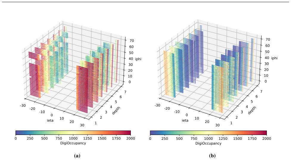
- [Sec. 3] The reported percentage changes (60% reduction, 188% increase) should be double-checked against the plotted mean DigiOccupancy values; the 188% increase description seems inconsistent with the downward trend within a run described in the same paragraph.
- [Figs. 8-9] The figure captions refer to 'pointers' without explaining what they indicate; improve caption clarity.
- [Sec. 4.1, Eq. (4.1)] The notation for the conventional convolution is hard to follow (h', w', h'', w'' are not clearly defined). Consider using standard index notation.
- [Reference [29]] Reference [29] is cited as the source for the 40-degree HCAL power loss, but the title 'Search for disappearing tracks...' appears unrelated. Please verify the citation or replace it with the appropriate technical report.
Circularity Check
No significant circularity: the DepthViT derivation and ensemble evaluation are self-contained; the 'pristine validation data' requirement is an explicit scope condition, not a circular step.
full rationale
The claimed derivation chain is not circular. DepthViT is trained on a train split of a single run; mu_err and sigma_err are computed by applying the model to a separate validation split (Sec 5.1); synthetic anomalies are injected only into the test split (Sec 4.2, Sec 5.1). The Z-score detector (Eq. 4.11) and gap-score rule (Eqs. 4.12, G0=0.3) are then evaluated on test data that was not used to compute the baseline statistics. The continual-learning results in Sec 5.3 are honest comparisons: updating mu/sigma from each run's validation set, training new ensemble members, and testing on that run's test set with injected anomalies. No fitted parameter is fed back as the predicted target. The explicit statement that the method 'relies solely on the continued availability of pristine detector data' (Sec 5.3) is a genuine limitation for live DQM streams, since contamination of the validation data would absorb anomalies into the baseline; however, this is an external assumption about deployment data quality, not a circular definition or a fitted quantity renamed as prediction. The threshold G0 is optimized once, which is a model-selection/generalization concern rather than circularity. There are no load-bearing self-citations or imported uniqueness theorems.
Assumptions & free parameters
free parameters (9)
- G0 (gap-score threshold) =
0.3
- Time window T =
5 lumisections
- Patch size =
12
- Number of kernels =
8
- Mask ratio =
0.5
- Number of layers =
5
- Latent dimension =
56
- Ensemble size =
4 runs
- Quantile-scaling epsilon =
unspecified small value
assumptions (5)
- domain assumption Synthetic single-pixel multiplicative anomalies (factors 0.0-2.0) faithfully mimic real HCAL dead, degraded, and hot channels.
- domain assumption Pristine, anomaly-free validation data is available for every new run to update mu_err/sigma_err and to train new models.
- domain assumption Only a single anomaly per lumisection needs to be detected.
- standard math Per-pixel prediction errors for pristine data are approximately independent and identically distributed so Eq. 4.11 follows a standard normal under the null.
- domain assumption A sliding window of the four most recent runs is sufficient to span the relevant distribution-shift regime.
Cite this review
Pith. "Pith review of Continual Learning via Ensemble-Based Depth-Wise Masked Autoencoders for Data Quality Monitoring in High-Energy Physics." pith.science (2026). https://pith.science/paper/YQPYN3LO
@misc{pith2026260302369,
  author       = {Pith},
  title        = {Pith review of: Continual Learning via Ensemble-Based Depth-Wise Masked Autoencoders for Data Quality Monitoring in High-Energy Physics},
  year         = {2026},
  howpublished = {\url{https://pith.science/paper/YQPYN3LO}},
  note         = {Machine review of arXiv:2603.02369}
}
read the original abstract
Machine learning (ML) techniques have been demonstrated to improve the accuracy and efficiency of anomaly detection (AD) when compared to conventional methods. This has led to the adoption of ML for data quality monitoring (DQM) use cases in order to monitor the operation of certain systems to ensure that they are free of undesirable or potentially deleterious anomalies. For applications in the field of High-Energy physics (HEP), where detectors must operate in long-running, harsh environments, ML models used in DQM that have been trained on static datasets are bound to experience degraded performance due to distributional shifts that naturally occur in the incoming data streams, unless directly mitigated via the inclusion of continual ML techniques. This work introduces DepthViT, a lightweight masked autoencoder architecture that employs unique depth-wise embeddings and depth-wise attention, to perform computationally efficient AD tasks. A continual learning framework is developed in which DepthViT models trained on the most recent data streams are ensembled with older models to create a robust overall system which is more resilient to shifts in incoming data streams. When evaluated on occupancy maps from the Compact Muon Solenoid (CMS) hadron calorimeter across multiple data-taking campaigns, the proposed method maintains precision above 98.8\% and a stable ratio of correct anomaly predictions to number of anomalies both under small and large distributional shifts. Beyond HEP, the same ensembling-based continual adaptation strategy can be directly applied to industrial monitoring environments where data also naturally evolve over time. This work therefore presents a path toward adaptive anomaly detection systems capable of sustained operation in dynamic data environments.
Figures


Figures from the paper (5 more)


Reference graph
Works this paper leans on
-
[6]
Spatio-Temporal Anomaly Detection with Graph Networks for Data Quality Mon- itoring of the Hadron Calorimeter,
M. W. Asres et al., “Spatio-Temporal Anomaly Detection with Graph Networks for Data Quality Mon- itoring of the Hadron Calorimeter,”Sensors, vol. 23, no. 24, 2023,ISSN: 1424-8220.DOI:10.3390/ s23249679
2023
-
[8]
Data Quality Monitoring for the Hadron Calorimeters Using Transfer Learning for Anomaly Detection,
M. W. Asres et al., “Data Quality Monitoring for the Hadron Calorimeters Using Transfer Learning for Anomaly Detection,”Sensors, vol. 25, no. 11, 2025,ISSN: 1424-8220.DOI:10.3390/s25113475
-
[1]
Scientific discovery in the age of artificial intelligence,
H. Wang et al., “Scientific discovery in the age of artificial intelligence,”Nature, vol. 620, no. 7972, pp. 47–60, 2023,ISSN: 1476-4687.DOI:10.1038/s41586-023-06221-2 16
-
[2]
A Comprehensive Investigation of Anomaly Detection Methods in Deep Learning and Machine Learning: 2019–2023,
S. Kumari, C. Prabha, A. Karim, M. M. Hassan, and S. Azam, “A Comprehensive Investigation of Anomaly Detection Methods in Deep Learning and Machine Learning: 2019–2023,”IET Information Security, vol. 2024, no. 1, p. 8 821 891, 2024.DOI:https : / / doi . org / 10 . 1049 / 2024 / 8821891
2019
-
[3]
The Data Quality Monitoring Software for the CMS experiment at the LHC: past, present and future,
Azzolini, Virginia et al., “The Data Quality Monitoring Software for the CMS experiment at the LHC: past, present and future,”EPJ Web Conf., vol. 214, p. 02 003, 2019.DOI:10 . 1051 / epjconf / 201921402003
2019
-
[4]
Machine Learning Anomaly Detection Applications to Compact Muon Solenoid Data Qual- ity Monitoring,
A. A. Pol, “Machine Learning Anomaly Detection Applications to Compact Muon Solenoid Data Qual- ity Monitoring,” Theses, Universit´e Paris-Saclay, Jun. 2020. [Online]. Available:https://theses. hal.science/tel-02924477
2020
-
[5]
Machine learning for anomaly detection in particle physics,
V . Belis, P. Odagiu, and T. K. Aarrestad, “Machine learning for anomaly detection in particle physics,” Reviews in Physics, vol. 12, p. 100 091, 2024,ISSN: 2405-4283.DOI:https : / / doi . org / 10 . 1016/j.revip.2024.100091
arXiv 2024
-
[7]
Long Horizon Anomaly Prediction in Multivariate Time Series with Causal Autoen- coders,
M. W. Asres et al., “Long Horizon Anomaly Prediction in Multivariate Time Series with Causal Autoen- coders,”PHM Society European Conference, vol. 7, no. 1, pp. 21–31, 2022.DOI:10.36001/phme. 2022.v7i1.3367
Show all 33 references
-
[9]
The upgrade of the CMS hadron calorimeter with silicon photomultipliers,
N. Strobbe, “The upgrade of the CMS hadron calorimeter with silicon photomultipliers,”Journal of Instrumentation, vol. 12, no. 01, p. C01080, Jan. 2017.DOI:10 . 1088 / 1748 - 0221 / 12 / 01 / C01080
2017
-
[10]
LHC Machine,
L. Evans and P. Bryant, “LHC Machine,”Journal of Instrumentation, vol. 3, no. 08, S08001, Aug. 2008. DOI:10.1088/1748-0221/3/08/S08001
2008 doi
-
[11]
The CMS experiment at the CERN LHC,
CMS Collaboration, “The CMS experiment at the CERN LHC,”Journal of Instrumentation, vol. 3, no. 08, S08004, Aug. 2008.DOI:10.1088/1748-0221/3/08/S08004
2008 doi
-
[12]
CMS Technical Design Report for the Phase 1 Upgrade of the Hadron Calorimeter,
J. Mans et al., “CMS Technical Design Report for the Phase 1 Upgrade of the Hadron Calorimeter,” CERN, Tech. Rep., 2012. [Online]. Available:https://cds.cern.ch/record/1481837
2012
-
[13]
The CMS trigger system,
CMS Collaboration, “The CMS trigger system,”Journal of Instrumentation, vol. 12, no. 01, P01020, Jan. 2017.DOI:10.1088/1748-0221/12/01/P01020
2017 doi
-
[14]
Characteristics of the ATLAS and CMS detectors,
A. Seiden, “Characteristics of the ATLAS and CMS detectors,”Philosophical Transactions of the Royal Society A: Mathematical, Physical and Engineering Sciences, vol. 370, pp. 892–906, 2012.DOI:10. 1098/rsta.2011.0461
2012
-
[15]
CMS data quality monitoring: Systems and experi- ences,
L. Tuura, A. Meyer, I. Segoni, and G. D. Ricca, “CMS data quality monitoring: Systems and experi- ences,”Journal of Physics: Conference Series, vol. 219, no. 7, p. 072 020, Apr. 2010.DOI:10.1088/ 1742-6596/219/7/072020
2010
-
[16]
Overcoming catastrophic forgetting in neural networks,
J. Kirkpatrick et al., “Overcoming catastrophic forgetting in neural networks,”Proceedings of the Na- tional Academy of Sciences, vol. 114, no. 13, pp. 3521–3526, 2017.DOI:10.1073/pnas.1611835114 17
2017 doi
-
[17]
Continual learning through synaptic intelligence,
F. Zenke, B. Poole, and S. Ganguli, “Continual learning through synaptic intelligence,” inProceed- ings of the 34th International Conference on Machine Learning, ser. Proceedings of Machine Learning Research, vol. 70, PMLR, 2017, pp. 3987–3995
2017
-
[18]
Gradient episodic memory for continual learning,
D. Lopez-Paz and M. Ranzato, “Gradient episodic memory for continual learning,” inAdvances in Neural Information Processing Systems, vol. 30, 2017, pp. 6467–6476
2017
-
[19]
Icarl: Incremental classifier and represen- tation learning,
S.-A. Rebuffi, A. Kolesnikov, G. Sperl, and C. H. Lampert, “Icarl: Incremental classifier and represen- tation learning,” inProceedings of the IEEE Conference on Computer Vision and Pattern Recognition, 2017, pp. 5533–5542.DOI:10.1109/CVPR.2017.587
2017 doi
-
[20]
Progressive neural networks,
A. A. Rusu et al., “Progressive neural networks,”arXiv preprint arXiv:1606.04671, 2016
2016 arXiv
-
[21]
Packnet: Adding multiple tasks to a single network by iterative pruning,
A. Mallya and S. Lazebnik, “Packnet: Adding multiple tasks to a single network by iterative pruning,” inProceedings of the IEEE Conference on Computer Vision and Pattern Recognition, 2018, pp. 7765– 7773.DOI:10.1109/CVPR.2018.00810
2018
-
[22]
I. E. Marouf, S. Roy, E. Tartaglione, and S. Lathuili `ere,Weighted Ensemble Models Are Strong Contin- ual Learners, 2024. arXiv:2312.08977 [cs.LG]. [Online]. Available:https://arxiv.org/ abs/2312.08977
2024 arXiv
-
[23]
T. Doan, S. I. Mirzadeh, and M. Farajtabar,Continual Learning Beyond a Single Model, 2023. arXiv: 2202.09826 [cs.LG]. [Online]. Available:https://arxiv.org/abs/2202.09826
2023 arXiv
-
[24]
Zhou, H.-L
D.-W. Zhou, H.-L. Sun, H.-J. Ye, and D.-C. Zhan,Expandable Subspace Ensemble for Pre-Trained Model-Based Class-Incremental Learning, 2024. arXiv:2403.12030 [cs.CV]. [Online]. Available: https://arxiv.org/abs/2403.12030
2024 arXiv
-
[25]
W ´ojcik, W
M. W ´ojcik, W. Ko´sciukiewicz, T. Kajdanowicz, and A. Gonczarek,Neural Architecture for Online En- semble Continual Learning, 2023. arXiv:2211 . 14963 [cs.LG]. [Online]. Available:https : //arxiv.org/abs/2211.14963
2023 arXiv
-
[26]
Rype ´s´c, S
G. Rype ´s´c, S. Cygert, V . Khan, T. Trzci´nski, B. Zieli ´nski, and B. Twardowski,Divide and not forget: Ensemble of selectively trained experts in Continual Learning, 2024. arXiv:2401.10191 [cs.LG]. [Online]. Available:https://arxiv.org/abs/2401.10191
2024 arXiv
-
[27]
Ye and A
F. Ye and A. G. Bors,Learning an evolved mixture model for task-free continual learning, 2022. arXiv: 2207.05080 [cs.LG]. [Online]. Available:https://arxiv.org/abs/2207.05080
2022 arXiv
-
[28]
O. S. Br ¨uning et al.,LHC Design Report(CERN Yellow Reports: Monographs). Geneva: CERN, 2004. DOI:10.5170/CERN-2004-003-V-1
2004 doi
-
[29]
Search for disappearing tracks in proton-proton collisions at √s= 13 TeV,
The CMS Collaboration, “Search for disappearing tracks in proton-proton collisions at √s= 13 TeV,” Physics Letters B, vol. 806, p. 135 502, 2020,ISSN: 0370-2693.DOI:https : / / doi . org / 10 . 1016/j.physletb.2020.135502
2020
-
[30]
Dosovitskiy et al.,An Image is Worth 16x16 Words: Transformers for Image Recognition at Scale,
A. Dosovitskiy et al.,An Image is Worth 16x16 Words: Transformers for Image Recognition at Scale,
-
[31]
K. He, X. Chen, S. Xie, Y . Li, P. Doll ´ar, and R. Girshick,Masked Autoencoders Are Scalable Vision Learners, 2021. arXiv:2111 . 06377 [cs.CV]. [Online]. Available:https : / / arxiv . org / abs/2111.06377 18
2021 arXiv
-
[32]
Ristea, F.-A
N.-C. Ristea, F.-A. Croitoru, R. T. Ionescu, M. Popescu, F. S. Khan, and M. Shah,Self-distilled masked auto-encoders are efficient video anomaly detectors, 2024. arXiv:2306.12041 [cs.CV]. [Online]. Available:https://arxiv.org/abs/2306.12041 19 The CMS HCAL Collaboration Yereva...
2024 arXiv
- [2021]
Reviewed August 2, 2026 · model on record in the stance chip above.
Discussion (0). Sign in to comment.