Quasi-optimal sampling from Gibbs states via non-commutative optimal transport metrics
Pith reviewed 2026-05-23 07:52 UTC · model grok-4.3
The pith
Gibbs states of local commuting Hamiltonians that satisfy decay of matrix-valued quantum conditional mutual information can be quasi-optimally prepared on quantum computers by controlling Davies evolution mixing in a normalized quantum Wass
A machine-rendered reading of the paper's core claim, the machinery that carries it, and where it could break.
Core claim
Any Gibbs state of a local commuting Hamiltonian on a hypercubic lattice that obeys decay of matrix-valued quantum conditional mutual information can be quasi-optimally prepared by controlling the mixing time of the associated Davies evolution in a normalized quantum Wasserstein distance of order one.
What carries the argument
Decay of matrix-valued quantum conditional mutual information (MCMI), which supplies the weak approximate tensorization and the new weak transport cost inequality that bound the Wasserstein mixing time.
If this is right
- Quantum CSS codes at high temperature admit effective local Hamiltonians, satisfy MCMI decay, and are therefore quasi-optimally preparable.
- Under an extra local gap assumption the same method gives rapid trace-distance mixing for interaction ranges beyond two.
- The normalized quantum Wasserstein distance of order one becomes a practical tool for proving rapid mixing of quantum thermalizing dynamics.
- Quasi-optimal sampling from such Gibbs states is possible on a quantum computer without requiring stronger clustering assumptions.
Where Pith is reading between the lines
- MCMI decay may serve as a verifiable proxy for efficient preparability in other quantum many-body models beyond the commuting case.
- The non-commutative transport metric could be applied to mixing analyses of open quantum systems outside the Gibbs setting.
- Checking MCMI decay on finite lattices might be computationally cheaper than verifying other known clustering conditions.
Load-bearing premise
The Gibbs state must satisfy the newly introduced decay of matrix-valued quantum conditional mutual information condition.
What would settle it
A concrete local commuting Hamiltonian whose Gibbs state violates MCMI decay yet whose Davies evolution still achieves the claimed quasi-optimal Wasserstein mixing time, or conversely a system obeying MCMI decay whose mixing time fails to be quasi-optimal.
Figures


read the original abstract
We study the problem of sampling from and preparing quantum Gibbs states of local commuting Hamiltonians on hypercubic lattices of arbitrary dimension. We prove that any such Gibbs state which satisfies a clustering condition that we coin decay of matrix-valued quantum conditional mutual information (MCMI) can be quasi-optimally prepared on a quantum computer. We do this by controlling the mixing time of the corresponding Davies evolution in a normalized quantum Wasserstein distance of order one. To the best of our knowledge, this is the first time that such a non-commutative transport metric has been used in the study of quantum dynamics, and the first time quasi-rapid mixing is implied by solely an explicit clustering condition. Our result is based on a weak approximate tensorization and a weak modified logarithmic Sobolev inequality for such systems, as well as a new general weak transport cost inequality. If we furthermore assume a constraint on the local gap of the thermalizing dynamics, we obtain rapid mixing in trace distance for interactions beyond the range of two, thereby extending the state-of-the-art results that only cover the nearest neighbor case. We conclude by showing that systems that admit effective local Hamiltonians, like quantum CSS codes at high temperature, satisfy this MCMI decay and can thus be efficiently prepared and sampled from.
Editorial analysis
A structured set of objections, weighed in public.
Referee Report
Summary. The manuscript proves that Gibbs states of local commuting Hamiltonians on hypercubic lattices satisfying a decay condition on matrix-valued quantum conditional mutual information (MCMI) admit quasi-optimal preparation on a quantum computer. This is achieved by bounding the mixing time of the associated Davies evolution in a normalized quantum Wasserstein distance of order one. The argument rests on a weak approximate tensorization property, a weak modified logarithmic Sobolev inequality, and a new weak transport-cost inequality. Under an additional local-gap assumption the result upgrades to rapid mixing in trace distance for interactions of range greater than two. The MCMI condition is verified for high-temperature CSS codes, which therefore admit efficient preparation and sampling.
Significance. If the derivations are correct, the work is significant because it supplies the first explicit clustering condition (MCMI decay) that implies quasi-rapid mixing for quantum Gibbs states, employs a non-commutative optimal-transport metric for the first time in the analysis of quantum dynamics, and extends rapid-mixing guarantees beyond nearest-neighbor interactions. The concrete verification for CSS codes indicates immediate applicability to quantum error-correcting codes at high temperature. The combination of weak tensorization, weak mLSI, and a new transport inequality constitutes a technically coherent advance in the study of quantum thermalization.
minor comments (2)
- The abstract states that the result is 'to the best of our knowledge' the first use of a non-commutative transport metric for quantum dynamics; a brief comparison paragraph in the introduction with the classical Wasserstein literature and the few existing quantum-Wasserstein papers would strengthen this claim.
- Notation for the normalized quantum W_1 distance and the precise definition of 'quasi-optimal' mixing time should be introduced with a dedicated paragraph or displayed equation in Section 2 (Preliminaries) rather than only in the technical sections.
Simulated Author's Rebuttal
We thank the referee for their positive assessment of the manuscript, recognition of its significance, and recommendation to accept. No major comments were raised in the report.
Circularity Check
No significant circularity; derivation conditional on explicit MCMI assumption
full rationale
The paper's central result is an implication: MCMI decay (newly coined clustering condition) plus weak approximate tensorization, weak mLSI, and a new weak transport-cost inequality imply quasi-optimal mixing in normalized quantum W_1 distance for Davies evolution. MCMI is introduced as an assumption, not derived from the target mixing bound; it is separately verified for high-temperature CSS codes. No self-citations are load-bearing for the main theorem, no parameters are fitted then renamed as predictions, and no ansatz or uniqueness claim reduces to prior author work by construction. The argument is self-contained against the stated hypotheses.
Axiom & Free-Parameter Ledger
axioms (2)
- domain assumption Davies evolution generates a valid quantum Markov semigroup for local commuting Hamiltonians
- domain assumption Weak approximate tensorization and weak modified logarithmic Sobolev inequality hold under MCMI decay
invented entities (1)
-
Matrix-valued quantum conditional mutual information (MCMI) decay
no independent evidence
Forward citations
Cited by 1 Pith paper
-
Quantum Gibbs sampling through the detectability lemma
Detectability lemma enables Gibbs sampling without Lindbladian simulation, yielding O(M) cost reduction for M-term local Lindbladians and quadratic speedup in spectral gap for frustration-free and commuting cases.
Reference graph
Works this paper leans on
-
[1]
[AFH09] R Alicki, M Fannes, and M Horodecki
doi:10.1109/focs.2011.58. [AFH09] R Alicki, M Fannes, and M Horodecki. On thermalization in kitaev’s 2d model. Journal of Physics A: Mathematical and Theoretical , 42(6):065303, January 2009. doi:10.1088/1751-8113/42/6/065303. [AJK+21a] Nima Anari, Vishesh Jain, Frederic Koehler, Huy Tuan Pham, and Thuy-Duong Vuong. Entropic independence i: Modified log-s...
-
[2]
[BCPH24] Andreas Bluhm, ´Angela Capel, and Antonio P´ erez-Hern´ andez
doi:10.22331/q-2022-02-10-650 . [BCPH24] Andreas Bluhm, ´Angela Capel, and Antonio P´ erez-Hern´ andez. Strong decay of correlations for gibbs states in any dimension, 2024. doi:10.48550/ARXIV.2401. 10147. [BCR21] Ivan Bardet, ´Angela Capel, and Cambyse Rouz´ e. Approximate tensorization of the relative entropy for noncommuting conditional expectations. A...
-
[3]
doi:10.48550/ARXIV.2410.10495. [BK18] Fernando G. S. L. Brand˜ ao and Michael J. Kastoryano. Finite correlation length implies efficient preparation of quantum thermal states. Communications in Math- ematical Physics, 365(1):1–16, May 2018. doi:10.1007/s00220-018-3150-8. [BLMT24] Ainesh Bakshi, Allen Liu, Ankur Moitra, and Ewin Tang. High-temperature gibb...
-
[4]
Literaturverz. S. 161 - 167. [Dav79] E.B. Davies. Generators of dynamical semigroups. Journal of Functional Analysis , 34(3):421–432, December 1979. doi:10.1016/0022-1236(79)90085-5. [DLL24] Zhiyan Ding, Bowen Li, and Lin Lin. Efficient quantum gibbs samplers with kubo– martin–schwinger detailed balance condition, 2024. doi:10.48550/ARXIV.2404. 05998. 14 ...
-
[5]
[DPR22] Giacomo De Palma and Cambyse Rouz´ e
doi:10.48550/ARXIV.2403.18617. [DPR22] Giacomo De Palma and Cambyse Rouz´ e. Quantum concentration inequali- ties. Annales Henri Poincar´ e, 23(9):3391–3429, April 2022. doi:10.1007/ s00023-022-01181-1. [DS85] R. L. Dobrushin and S. B. Shlosman. Completely Analytical Gibbs Fields , pages 371–403. Birkh¨ auser Boston, 1985.doi:10.1007/978-1-4899-6653-7_21 ...
-
[6]
[FLT24] Di Fang, Jianfeng Lu, and Yu Tong
doi:10.1038/s41467-024-51592-3. [FLT24] Di Fang, Jianfeng Lu, and Yu Tong. Mixing time of open quantum systems via hypocoercivity, 2024. doi:10.48550/ARXIV.2404.11503. [GCDK24] Andr´ as Gily´ en, Chi-Fang Chen, Joao F. Doriguello, and Michael J. Kastoryano. Quantum generalizations of glauber and metropolis dynamics, 2024. doi:10.48550/ ARXIV.2405.20322. [...
-
[7]
E∗ N (X) = X for all X ∈ N
-
[8]
E∗ N (V XW ) = V E ∗ N (X)W for all V, W ∈ N and X ∈ B(H). For such conditional expectations, the relative entropy exhibits special properties known as the chain rule and exact entropy factorization: given conditional expectation E∗ N : B(H) → N and E∗ M : B(H) → B(H) with [E∗ M, E∗ N ] = 0, the chain rule states that for any stateσ = EN (σ) ∈ S (H), and ...
-
[9]
Commutativity: All terms hA ⊗ I A, A ⊆ Λ pairwise commute
-
[10]
( κ, r)-locality: hA = 0 if either |A| > κ or diam(A) > r
-
[11]
Bounded interaction strength: max A⊆Λ ∥hA∥∞ =: J < ∞
-
[12]
22 Note that the growth constant g is a function of κ, r and D, and that κ, r are not independent
Bounded connectivity: max k∈Λ |{A ⊆ Λ : hA ̸= 0, k ∈ A}| =: g < ∞. 22 Note that the growth constant g is a function of κ, r and D, and that κ, r are not independent. Despite that, we will treat them in this work as separate parameters. When considering a family of Hamiltonians on increasing lattice sizes, such as those arising from an interaction on ZD, a...
-
[13]
E∅ = id and EΛ = tr[ · ] σΛ
-
[14]
for each A ⊂ A∂ ⊆ B ⊆ Λ, σB is a fixed point of EA
-
[15]
for each A ⊆ B ⊆ Λ, EAEB = EBEA = EB
-
[16]
Note that here and in the following we will use ⊔ to denote a disjoint union of sets
for any two regions A, B ⊆ Λ such that A∂ ∩ B∂ = ∅, EA⊔B = EAEB = EBEA, that will become useful later. Note that here and in the following we will use ⊔ to denote a disjoint union of sets. By using the representation EA = lim t→∞ Rn σ,A , (33) in terms of the Petz recovery RA,σ(X) := σ1/2(σ−1/2 A trA[X]σ−1/2 A ) ⊗ I A σ1/2 , proven in [BCR21, Theorem 1] a...
-
[17]
˜hA X is supported in X ∩ A for every X ⊆ Λ
-
[18]
For A′ ⊆ Λ, ˜hA X = ˜hA′ X for all X ⊆ Λ for which X ∩ A′ = X ∩ A
-
[19]
One has log d−1 A I A ⊗ trA[e−βHΛ] = P X⊆Λ ˜hA X = ˜H A. The existence of an effective Hamiltonian alone does not suffice to ensure the decay of the MCMI, as the above definition lacks information on the system’s locality. In general, this decay will require an additional locality assumption (see Appendix D.1). However, when the system Hamiltonian is also...
-
[20]
c ∈ N with c ≥ r the overlap length , ensuring a sufficiently fast decay when using a weak approximate tensorization to consecutively cut out cells reducing the extensive dimension in every step
-
[21]
k ∈ N with k ≥ r the buffer length, separating cells of the same dimensionality such that the corresponding conditional expectations commute and hence allow us to use tensorization of the relative entropy
-
[22]
ℓ ∈ N with L ≥ ℓ and ℓ odd the ‘extensive’ side length of the cells we decompose into. As we will consecutively reduce the ‘extensive’ dimensions until we reach zero subtracting ℓ in every step by 2( k + c), we further require ℓ > 2D(k + c). Remark 3. In the first step of the decomposition, we aim to divide Λ L into hypercubes of side length ℓ. This might...
-
[23]
The interior of C∂ D,i, excluding a boundary layer of buffer length k: CD,i := {v ∈ C∂ D,i : dist( v, C∂ D,i) > k }
-
[24]
In the above R ⊆ ΛL is given by R = ΛL\R
A further restricted interior, excluding a boundary layer of width k + c, i.e excluding buffer and overlap length: ˚CD,i := {v ∈ C∂ D,i : dist( v, C∂ D,i) > k + c} . In the above R ⊆ ΛL is given by R = ΛL\R. We define the aggregate sets: CD := G i∈ID CD,i ˚CD := G i∈ID ˚CD,i, whereF denotes the disjoint union. Finally, we set CD−1 := ΛL \ ˚CD. For a visua...
-
[25]
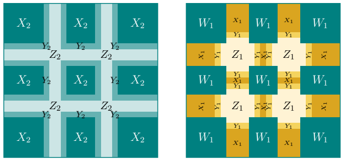
First, we identify the set of vertices that “join” each pair of neighbouring ˚Ca+1,i: C∂ a := v ∈ Ca : ∃j ∈ Z, b ∈ J1, DK : v + jeb ∈ Ca . 30 C ∂ 2,1 C ∂ 2,2 C ∂ 2,3 C ∂ 2,4 C ∂ 2,6 C ∂ 2,7 C ∂ 2,8 C ∂ 2,9 5 C ∂ 2,5 C2,5 ˚C2,5 ℓ kc ΛL ⊂ Z2 ˚C2 ˚C2 ˚C2 ˚C2 ˚C2 ˚C2 ˚C2 ˚C2 ˚C2 C2 C2 C2 C2 C2 C2 C2 C2 ΛL 2L+ 1 Figure 4: Splitting of Λ L = CD for D = 2 as des...
-
[26]
By construction, C∂ a is a disjoint union of fattened a-cells, which we denote as C∂ a,i with index set I a
-
[27]
We set the aggregated sets to be Ca := G i∈Ia Ca,i , ˚Ca := G i∈Ia ˚Ca,i
We again define the two subsets: Ca,i := {v ∈ C∂ a,i : dist( v, C∂ a,i ∩ Ca) > k } , ˚Ca,i := {v ∈ C∂ a,i : dist( v, C∂ a,i ∩ Ca) > k + c} separated from the skeleton that remains after removal of FD b=a+1 ˚Cb by buffer and overlap plus buffer length respectively. We set the aggregated sets to be Ca := G i∈Ia Ca,i , ˚Ca := G i∈Ia ˚Ca,i
-
[28]
Finally, we define the set for the next lower dimension: Ca−1 := Ca \ ˚Ca. This process is iterated for decreasing values of a, creating a hierarchical structure of cells of different extensive dimensions. For a visual representation of this construction for a = 1 in two dimensions (D = 2), refer to Figure 5. Lastly for a = 0 we set C0 := C1\˚C1 and ˚C0,i...
-
[29]
For each a ∈ J0, DK, ˚Ca :=F i∈Ia ˚Ca,i, Ca :=F i∈Ia Ca,i, and C∂ a :=F i∈Ia C∂ a,i are unions of disjoint sets, with size bounded as |˚Ca,i| ≤ | Ca,i| ≤ | C∂ a,i| ≤ ℓD.1 1This is a non-tight bound and it holds that |Ca,i| ≤ [2(D − a)(k + c)]D−a[ℓ − 2(D − a)(k + c)]a ≤ ℓD. 31 C∂ 1,1 C∂ 1,3 C∂ 1,6 C∂ 1,8 C∂ 1,11 C∂ 1,13 C∂ 1,2 C∂ 1,4 C∂ 1,7 C∂ 1,9 C∂ 1,12 ...
-
[30]
fat” 0-cells, in the shape of D-dimensional “crosses
C0 = C0 = ˚C0 =F i∈I0 C∂ 0,i is a disjoint union of “fat” 0-cells, in the shape of D-dimensional “crosses”, with each C∂ 0,i included in a hypercube of sidelength 2D(k + c) and distance dist(C∂ 0,i, C∂ 0,j) ≥ ℓ − 2D(k + c) > 0 from each other
-
[31]
SD a=0 Ca = CD = ΛL, and each site x ∈ ΛL is included in at most D + 1 sets {Ca,i}a,i
The hierarchy {Ca}D a=0 induces a suitably overlapping coarse-graining of ΛL, i.e. SD a=0 Ca = CD = ΛL, and each site x ∈ ΛL is included in at most D + 1 sets {Ca,i}a,i
-
[32]
c ≤ dist(Ca\Ca, ˚Ca) = dist(Ca\Ca, Ca\Ca−1) ∀a ∈ J1, DK,
-
[33]
For a visualization, find an example of the case D = 2 on the right side of Figure 6
2k ≤ dist(Ca,i, Ca,j) ∀i, j ∈ I a, ∀a ∈ J0, DK. For a visualization, find an example of the case D = 2 on the right side of Figure 6. 32 Proof. 1. We proceed by induction on a. For a = D, each of the sets C∂ D,i are hypercubes with sidelength ℓ, hence CD,i, ˚CD,i are hypercubes of side length at most ℓ − k and ℓ − (k + c), respectively. Disjointness is cl...
-
[34]
follows equally from the proof in 1
The disjointedness statement in 2. follows equally from the proof in 1. The statement C0 = ˚C0 follows by their definitions
-
[35]
We consider the following cases: Base case: If x ∈ CD, we are done
The proof proceeds by finite induction with at most D steps, starting from a = D. We consider the following cases: Base case: If x ∈ CD, we are done. Inductive step: If x /∈ CD, then x ∈ CD−1 ⊇ ΛL \ CD. For each subsequent step a, we have three possibilities: (a) If a = 0, then x /∈SD b=1 Cb. Consequently, x ∈ C0 = C∂ 0 = C0 = ˚C0, and we are done. (b) If...
-
[36]
Recall that k, c ≥ r, the range of the interactions. The claim follows via dist(Ca\Ca, ˚Ca) = dist(Ca\Ca,i, ˚Ca,i) = dist(Ca,i ∩ Ca, ˚Ca,i ∩ Ca) = dist({x ∈ Ca : dist(x, C∂ a,i) ≤ k}, {x ∈ Ca : dist(x, C∂ a,i) > k + c}) = c and it is easy to check that Ca\Ca−1 = Ca\(Ca\˚Ca) = ˚Ca for a ∈ J1, DK
-
[37]
This follows directly from the disjointness of Ca,i and Ca,j, see 1 . and their definition. 33 B.3 A weak approximate tensorization for Davies channels By combining the general weak entropy factorization from Appendix B.1 with the coarse-graining in Appendix B.2 this section contains a weak approximate tensorization (wAT) for the Davies channels with corr...
-
[38]
O poly log Nquasi-poly 1 ϵ2 poly log N ϵ2 = O poly log N, poly log 1 ϵ2 ancilla qubits,
-
[39]
O Nquasi-poly 1 ϵ2 poly log N ϵ2 = O Nquasi-log(N), quasi-poly(ϵ−2) two-qubit gates, block encodings of the Hamiltonian HΛ and the dissipative part of LD Λ . 45 Remark 6. Such algorithms are usually referred to as optimal if the complexity and/or runtime scales as O(N) up to polylogarithmic corrections. Since our scaling is O(N) up to quasi-logarithmic co...
discussion (0)
Sign in with ORCID, Apple, or X to comment. Anyone can read and Pith papers without signing in.