pith. sign in

arxiv: 2605.06648 · v2 · pith:572XD3AInew · submitted 2026-05-07 · 🌌 astro-ph.IM · astro-ph.EP

A preliminary exploration of the effects of baseline length for the LIFE space mission

Pith reviewed 2026-06-30 23:09 UTC · model grok-4.3

classification 🌌 astro-ph.IM astro-ph.EP
keywords LIFE missionnulling interferometrybaseline lengthexoplanet yieldhabitable planetsspace interferometryfringe trackingmission simulation
0
0 comments X

The pith

LIFE mission can restrict nulling baselines to 25-80m with under 10% loss in planet yield.

A machine-rendered reading of the paper's core claim, the machinery that carries it, and where it could break.

The paper tests whether the LIFE space mission's assumed 10-100 meter baseline range for nulling interferometry can be narrowed to ease spacecraft formation constraints. Using the LIFEsim simulator and updated planet occurrence rates, the authors compare planet detection yields and fringe tracking across different baseline sets. They conclude that a 25-80 meter range or even discrete baselines maintains performance within 10 percent. A new target-specific method for selecting optimal baselines is also presented. The result suggests mission design can trade some flexibility for simpler implementation.

Core claim

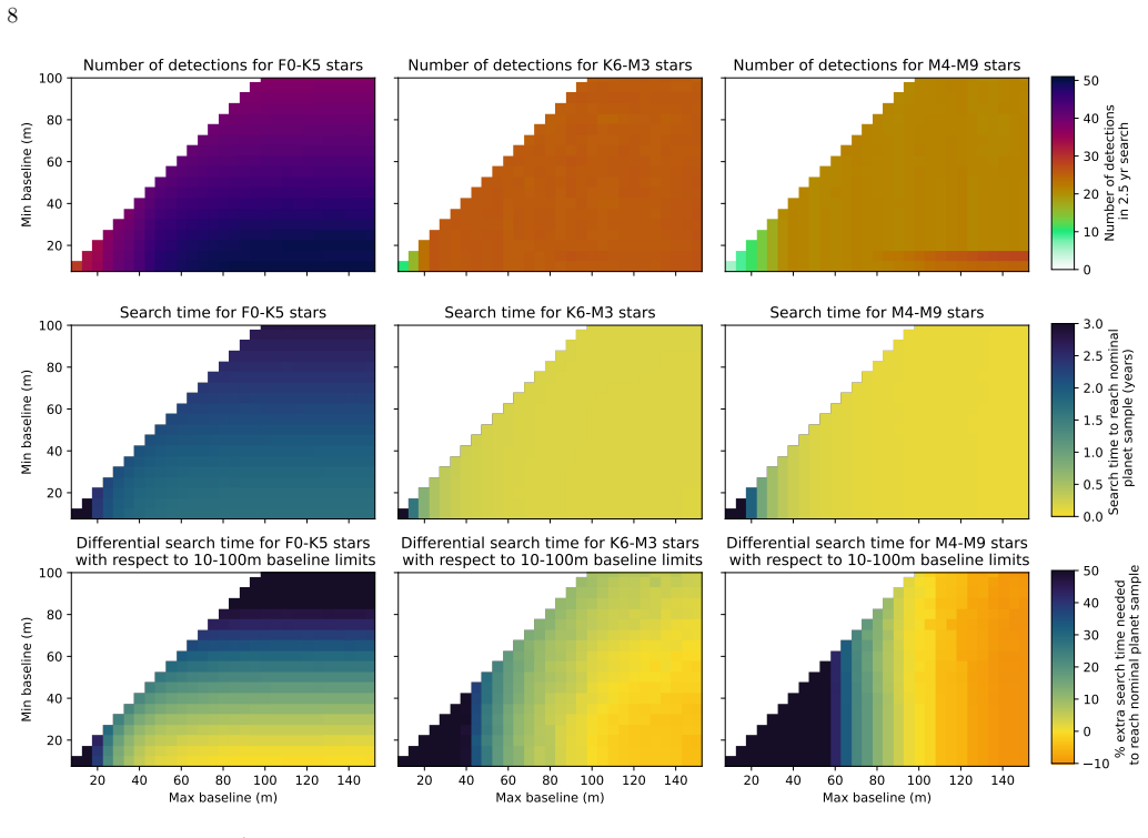
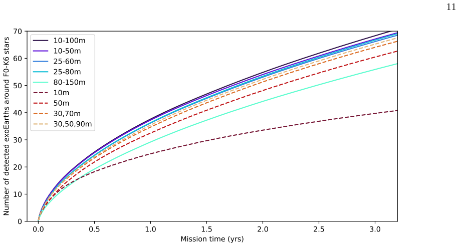
The authors determine that LIFE could utilise a considerably shorter range of baselines, such as 25-80m, or even discrete baselines without much (<10%) loss of performance, while also developing a new astrophysically motivated technique for choosing optimal baselines for a given science target.

What carries the argument

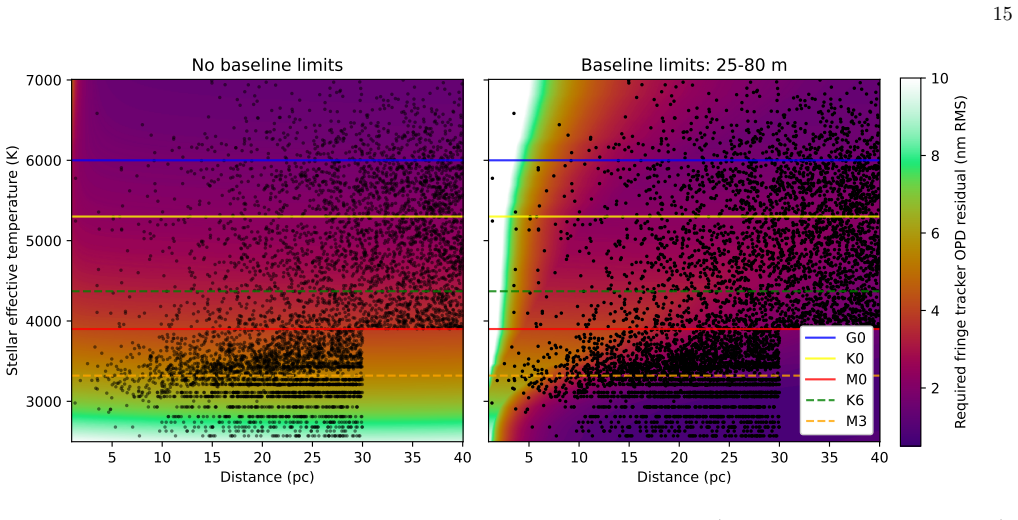
LIFEsim mission simulator used to quantify planet yield and fringe tracking performance across baseline length ranges.

If this is right

  • A baseline range of 25-80m delivers planet yields and tracking performance within 10 percent of the wider 10-100m range.
  • Discrete baseline sets can replace continuous ranges with comparable overall results.
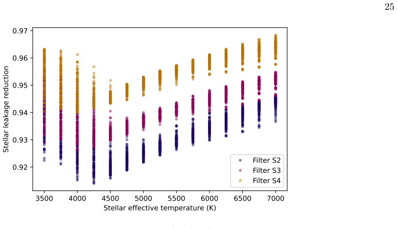
  • Spectral weighting requirements and target-specific optimization introduce necessary performance trade-offs.
  • Mission implementation can prioritize fewer baseline options without major science loss.

Where Pith is reading between the lines

These are editorial extensions of the paper, not claims the author makes directly.

  • Fewer baseline options could reduce the number of spacecraft or formation-keeping requirements.
  • The target-selection technique might apply to other nulling interferometry concepts beyond LIFE.
  • Incorporating measured noise spectra from prototype hardware would test the discrete-baseline claim directly.

Load-bearing premise

The LIFEsim simulator together with the revised planet occurrence statistics accurately capture real instrument performance and exoplanet populations across the parameter space explored.

What would settle it

Comparison of actual exoplanet detection counts from a deployed LIFE instrument against the simulated yields for 25-80m baselines, showing deviation beyond 10 percent.

Figures

Figures reproduced from arXiv: 2605.06648 by Adrian M. Glauser, Andrea Fortier, Felix A. Dannert, Jens Kammerer, Jonah T. Hansen, Lia Sartori, Philipp Huber, Romain Laugier, Sascha P. Quanz, Thomas Birbacher.

Figure 1
Figure 1. Figure 1: LIFEsim yield/mission time simulations for a range of baseline limits. The parameters for the simulation are detailed in the text, primarily section 4. The columns denote the three stellar samples in decreasing order of scientific priority. Top row: the raw yields for each baseline limit, given in planets detected. Middle row: the total amount of search time needed to find the nominal planet sample for eac… view at source ↗
Figure 2
Figure 2. Figure 2: The percentage of extra search time needed to fulfil the targets of all three stellar populations (50, 25 and 20 planets for stellar types F0-K5, K6-M3 and M4-M9 respectively) for a range of maximum and minimum baselines compared to the reference 10-100 m case. 5 10 15 20 25 30 35 40 Distance (pc) 3000 4000 5000 6000 7000 Stellar effective temperature (K) 1 10 24 24 96 96 1 10 10 24 24 96 96 G0 K0 M0 K6 M3… view at source ↗
Figure 3
Figure 3. Figure 3: Integration time required for an Earth-twin around a given star to reach an SNR of 7, plotted as a function of stellar parameters. The baseline limits are set at 25-80 m. The LIFE stellar sample is over-plotted in black, and integration time contours are over-plotted in white. Dotted contours show the same integration time contours, but for the 10-100 m case for comparative purposes. Solid horizontal lines… view at source ↗
Figure 4
Figure 4. Figure 4: The percentage of extra mission time that is needed compared to the flexible 10-100 m baseline array to detect the total number of planets specified in section 4 (50, 25 and 20 planets for stellar types F0-K5, K6-M3 and M4-M9 respectively), plotted for a variety of discrete baseline cases. Dashed contour lines at 10% and 20% are also displayed. The plot inset uses a much larger y-axis scaling to demonstrat… view at source ↗
Figure 5
Figure 5. Figure 5: Detection curve for a selection of baseline architectures, highlighting the cumulative number of exoEarth planet detections around solar-type stars as the mission unfolds. Baseline ranges are plotted as continuous lines, and discrete baselines as dashes. Having a single baseline of 10 m is incredibly problematic for the mission, resulting in a staggering 18 fold increase in mission time. Beyond the short, … view at source ↗
Figure 6
Figure 6. Figure 6: Integration time required for an Earth-twin around a given star to reach an SNR of 7, plotted as a function of stellar parameters, for two different discrete baseline configurations. The LIFE stellar sample is over-plotted in black, and integration time contours are over-plotted in white. Dotted contours show the same integration time contours, but for the 10-100 m baseline range case for comparative purpo… view at source ↗
Figure 7
Figure 7. Figure 7: Squared visibility as a function of stellar angular diameter and baseline. Over-plotted is the LIFE stellar catalogue, whereby we choose the nulling baseline to correspond to optimising against a planet at half the inner edge of the habitable zone. More than 95% of potential planets should lie at angular separations larger than this. The blue shaded region shows the 25-80 m nulling baseline range as discus… view at source ↗
Figure 8
Figure 8. Figure 8: Requirements on the fringe tracking residuals for a grid of stellar parameters (distance and effective temperature). The LIFE stellar catalogue within 40 pc is over-plotted in black. Solid horizontal lines show the boundaries between stellar types of F, G, K and M; and dashed horizontal lines show the boundaries between LIFE’s target stellar populations. Left: no restrictions on the baseline. Right: baseli… view at source ↗
Figure 9
Figure 9. Figure 9: Allowable fringe tracking bandwidth for varying stellar parameters. Overplotted in black is the LIFE catalog within 40 pc, and bandwidth contours are shown in white. A baseline limit of 25-80 m was imposed, and the OPD residuals were drawn from fig. 8. Solid horizontal lines show the boundaries between stellar types of F, G, K and M; and dashed horizontal lines show the boundaries between LIFE’s target ste… view at source ↗
Figure 10
Figure 10. Figure 10: Modulation efficiency curve of the Double Bracewell for varying aspect ratios as a function of off-axis angle. 2022; J. T. Hansen et al. 2022a), can be found at 0.59λ/B, and produces an average transmission of 0.55 telescope fluxes. The total planet flux is then the product of the planet’s spectral flux density Ep, the modulation efficiency, and the FOV taper function ρ(D, θ, λ), integrated over wavelengt… view at source ↗
Figure 11
Figure 11. Figure 11: The reduction in stellar leakage due to limb darkening (eq. (B21)) for various stellar models. Each point is an element of the table of parameters from A. Claret & S. Bloemen (2011), assuming the parameter cuts discussed in appendix B. The colours represent various Spitzer filters, with darker colours inferring shorter wavelengths. 3000 4000 5000 6000 7000 Stellar effective temperature (K) 0.0 0.1 0.2 0.3… view at source ↗
Figure 12
Figure 12. Figure 12 view at source ↗
Figure 13
Figure 13. Figure 13: Field of view coupling efficiency for a Gaussian and a uniform beam as a function of off-axis angle. Dashed lines indicate the outer working angle (50% of the maximum coupling efficiency). Left: linear scaling; Right: logarithmic scaling. 10 1 10 0 10 1 Off-axis angle (arcsec) 10 3 10 2 10 1 10 0 Collecting Power (AU) 3m, 4µm 2m, 4µm 1m, 4µm 0.5m, 4µm 3m, 10µm 2m, 10µm 1m, 10µm 0.5m, 10µm view at source ↗
Figure 14
Figure 14. Figure 14: Collecting power of different telescope sizes as a function of off-axis angle, arbitrarily scaled such that an on-axis source for a 3 m mirror is one. Shown for wavelengths of 4 µm (left) and 10 µm (right). Equivalent to the coupling efficiency plot in fig. 13 multiplied by the collecting area of the primary mirror. The off-axis coupling of a Gaussian beam into a single mode fibre is derived in Appendix A… view at source ↗
Figure 15
Figure 15. Figure 15: SNR for a variety of planet systems as a function of aperture diameter. EE refers to an ExoEarth twin at 1 AU, scaled by the square root of the stellar luminosity, and OHZ refers to an Earth placed at the outer edge of the habitable zone. A question arises as to whether it is advantageous to reduce (or stop-down) the aperture such that the increase in off-axis coupling efficiency overcomes the reduction i… view at source ↗
Figure 16
Figure 16. Figure 16: SNR as a function of baseline for various planet archetypes around a solar analogue star at 10 pc. Vertical dashed lines represent the optimal baseline for each case. 0 10 20 30 40 50 Baseline (m) 0 5 10 15 20 SNR 2 pc G dwarf at 0.2 AU 5 pc G dwarf at 0.5 AU 10 pc G dwarf at 1 AU 20 pc G dwarf at 2 AU 10 pc K dwarf at 1 AU 14.36 m 15.61 m 15.24 m 14.49 m 14.54 m view at source ↗
Figure 17
Figure 17. Figure 17: SNR as a function of baseline for different star archetypes considering an Earth analogue at 100 mas from the star. The first four lines are for a G2 dwarf at various distances (but holding angular separation constant) and the latter a cooler K7 dwarf at 10 pc. Vertical dashed lines represent the optimal baseline for each case. to see the effects of the limited FOV come into effect (hence why the star is … view at source ↗
Figure 18
Figure 18. Figure 18: SNR as a function of baseline multiplied by separation for an Earth twin around a solar analogue at 2 pc, shown for planets of varying separations. Vertical dashed lines represent the optimal baseline for each case. 10 1 10 2 10 3 Baseline (m) 1.0 0.5 0.0 0.5 1.0 Coefficient residual 1e 6 10 1 10 2 10 3 Baseline (m) 10 1 10 2 Baseline (m) view at source ↗
Figure 19
Figure 19. Figure 19: Residuals for each of the various MC parametric fits described in table 1 as a function of baseline. Left: Character￾isation model, with residual σ of 1.7 × 10⁻⁷ m rad, Middle: Kepler detection model, with residual σ of 5.9 × 10⁻⁸ m rad, Right: Uniform detection model, with residual σ of 4.4 × 10⁻⁸ m rad. The two detection models were run with fewer samples due to computational constraints. drawing insigh… view at source ↗
Figure 20
Figure 20. Figure 20: Number of exoplanet detections within the habitable zone for different baseline optimisations, stellar populations and statistical planet populations. The yields were run via LIFEsim (F. A. Dannert et al. 2022), with modifications described in the text. The various optimisation routines (shown in different colours) are: setting the “reference wavelength“ to 15 µm as previously done in LIFE yield papers; o… view at source ↗
read the original abstract

By aiming to find and characterise dozens of habitable exoplanets through the technique of nulling interferometry, the LIFE space mission will produce transformational science. One of the key parameters for such an interferometric mission is the nulling baseline length - the distance between nulled apertures, which past studies have assumed to be 10-100m. Advances in planet occurrence statistics and simulation tools allow us now to revisit this key assumption with significantly more detail, particularly with the intention to reduce the range of baselines considered due to mission implementation concerns. We utilise the LIFEsim mission simulator along with revised mathematical tools to identify whether the range of baselines could be reduced without significantly affecting planet yield and fringe tracking performance. Along the way, we also determine a new astrophysically motivated technique for choosing which baselines are optimal for a given science target. We find that indeed, LIFE could utilise a considerably shorter range of baselines, such as 25-80m, or even discrete baselines without much (<10%) loss of performance. Nevertheless, careful trade-offs between performance and implementation simplification must be made, especially considering any spectral weighting that may be required by the scientific goals, and the potential loss of target-specific baseline optimisation.

Editorial analysis

A structured set of objections, weighed in public.

Desk editor's note, referee report, simulated authors' rebuttal, and a circularity audit. Tearing a paper down is the easy half of reading it; the pith above is the substance, this is the friction.

Referee Report

2 major / 2 minor

Summary. The paper explores optimizing the nulling baseline length range for the LIFE space mission using the LIFEsim simulator and updated planet occurrence statistics. It concludes that restricting to 25-80 m (or discrete baselines) yields planet detection and fringe-tracking performance within <10% of the conventional 10-100 m range, while introducing an astrophysically motivated method for selecting target-specific optimal baselines.

Significance. If the simulation results hold under scrutiny, the finding could ease mission implementation constraints on baseline hardware without major scientific penalty. The use of revised occurrence rates and the simulator constitutes a clear update over prior studies; the new baseline-selection technique is a potentially reusable contribution if its derivation is made explicit.

major comments (2)
  1. [Methods / Simulation setup] The central <10% loss claim rests on LIFEsim outputs whose configuration (wavelength coverage, noise model, planet exclusion criteria, and error propagation) is not detailed enough to allow independent verification or sensitivity tests; this directly affects reproducibility of the yield tables.
  2. [Results] The post-hoc narrowing to 25-80 m (or discrete sets) is presented as performance-neutral, yet no quantitative comparison is shown for the full original range versus the restricted range across the same target sample; without this, the magnitude of any selection bias cannot be assessed.
minor comments (2)
  1. [Section 3] Notation for the new baseline-selection technique should be defined with an explicit equation or algorithm box rather than descriptive text only.
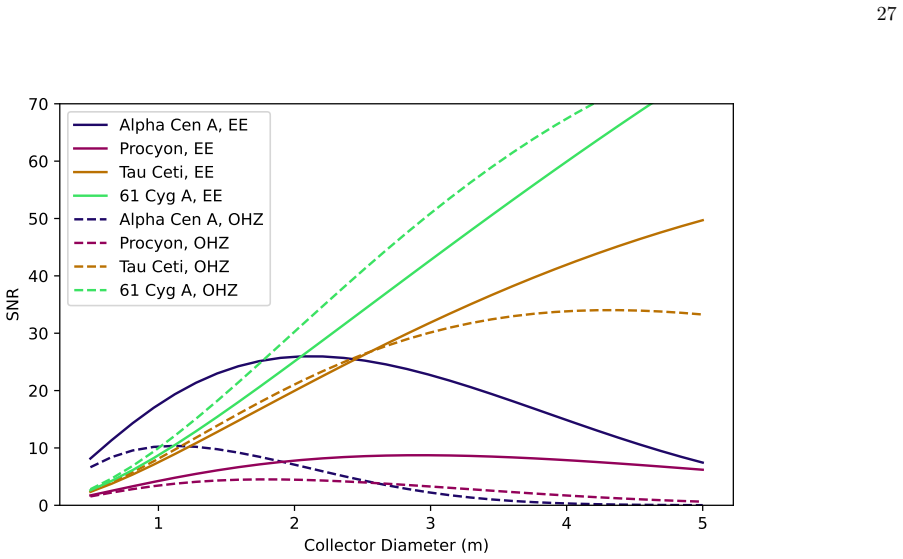
  2. [Figures 4-6] Figure captions should state the exact baseline sets compared and the number of simulated targets in each panel.

Simulated Author's Rebuttal

2 responses · 0 unresolved

We thank the referee for their thoughtful review and constructive comments, which have helped improve the clarity and reproducibility of our manuscript. We address each major comment below.

read point-by-point responses
  1. Referee: [Methods / Simulation setup] The central <10% loss claim rests on LIFEsim outputs whose configuration (wavelength coverage, noise model, planet exclusion criteria, and error propagation) is not detailed enough to allow independent verification or sensitivity tests; this directly affects reproducibility of the yield tables.

    Authors: We agree with the referee that more detailed information on the LIFEsim configuration is required to ensure reproducibility. In the revised version of the manuscript, we have substantially expanded the Methods section (Section 2) to include explicit details on the wavelength coverage (3-20 μm in 20 channels), the noise model (including photon noise, read noise, and background contributions), planet exclusion criteria (SNR > 5 for detection and characterization), and the error propagation methods used for yield calculations. We have also included a table summarizing the key simulation parameters and made the configuration files available as supplementary material. revision: yes

  2. Referee: [Results] The post-hoc narrowing to 25-80 m (or discrete sets) is presented as performance-neutral, yet no quantitative comparison is shown for the full original range versus the restricted range across the same target sample; without this, the magnitude of any selection bias cannot be assessed.

    Authors: The referee correctly notes that a direct quantitative comparison would be beneficial. Although our simulations inherently compared yields across different baseline ranges on the same target sample to derive the <10% loss figure, this was not presented explicitly in the original submission. We have now added a dedicated subsection in the Results (Section 3.2) with a new table and figure that directly compares the planet detection yields and fringe-tracking performance for the full 10-100 m range against the restricted 25-80 m range and discrete baseline sets, using the identical target list. These additions confirm the loss remains below 10% and allow assessment of any potential biases. revision: yes

Circularity Check

0 steps flagged

No significant circularity identified

full rationale

The paper reports simulation-based results from the external LIFEsim tool and revised occurrence statistics to assess baseline ranges and performance loss. No equations, derivations, or self-citation chains are shown that reduce the reported yields or <10% loss figures to quantities defined by the authors' own fitted parameters or prior ansatzes. The central claims rest on external simulator outputs rather than internal reductions, making the derivation self-contained against the provided text.

Axiom & Free-Parameter Ledger

0 free parameters · 2 axioms · 0 invented entities

The central claim rests on the fidelity of the LIFEsim simulator and the accuracy of updated planet occurrence statistics; these are external inputs whose validity is assumed rather than re-derived.

axioms (2)
  • domain assumption Updated planet occurrence statistics accurately reflect reality
    Invoked to justify revisiting the 10-100 m baseline assumption.
  • domain assumption LIFEsim correctly models nulling interferometry performance and fringe tracking
    Central to all yield and performance estimates.

pith-pipeline@v0.9.1-grok · 5782 in / 1298 out tokens · 36934 ms · 2026-06-30T23:09:14.679273+00:00 · methodology

discussion (0)

Sign in with ORCID, Apple, or X to comment. Anyone can read and Pith papers without signing in.

Reference graph

Works this paper leans on

3 extracted references

  1. [1]

    Stellar types of F through M (2500 K to 7000 K) 2.−1≤[F eH]≤1, chosen due to our targets lying in the solar neighbourhood (see e.g. M. Haywood (2001))

  2. [2]

    Log(g)≥3.5, derived from our stars being main sequence and the above stellar type range

  3. [3]

    outer working angle

    Microturbulence below 2 km/s, again from our stellar cut being relatively cool main sequence stars (see M. Steffen et al. (2013)) For the following analysis, we assume a parameterisation based on a quadratic relation as given in eq. (A6): LD(θ) = 1−a 1(1−µ)−a 2(1−µ) 2, µ= p 1−(2θ/δ s)2, θ≤δ s/2. To start with the limb darkening dependence on stellar leaka...