Geometric Analysis of the Damped Harmonic Oscillator via the Lambert W Function
Pith reviewed 2026-06-28 19:55 UTC · model grok-4.3
The pith
The Lambert W function supplies closed-form times for the underdamped oscillator to reach any amplitude threshold A via a logarithmic spiral mapping.
A machine-rendered reading of the paper's core claim, the machinery that carries it, and where it could break.
Core claim
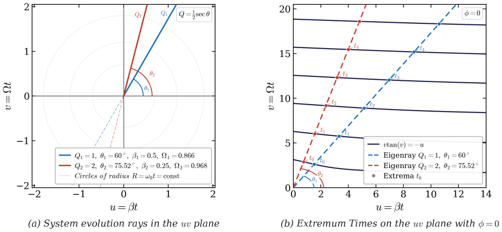
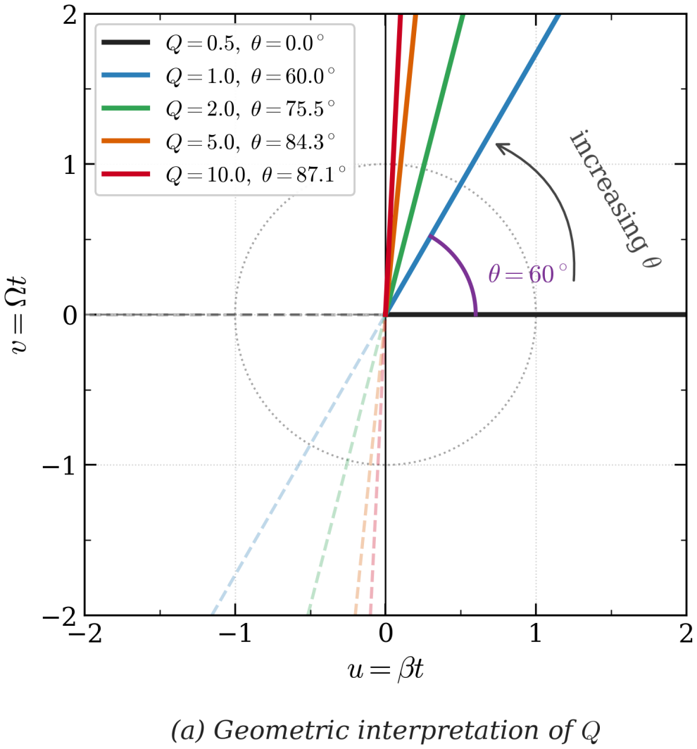
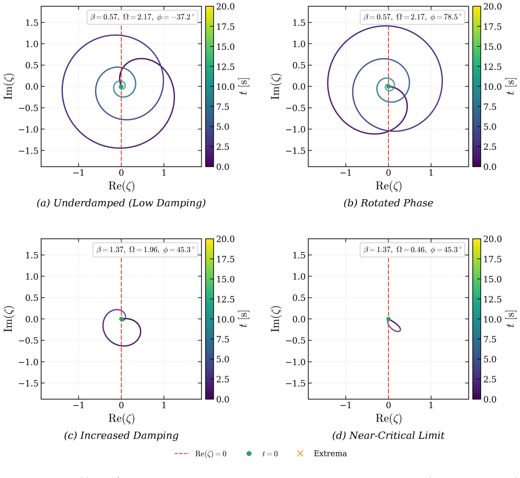
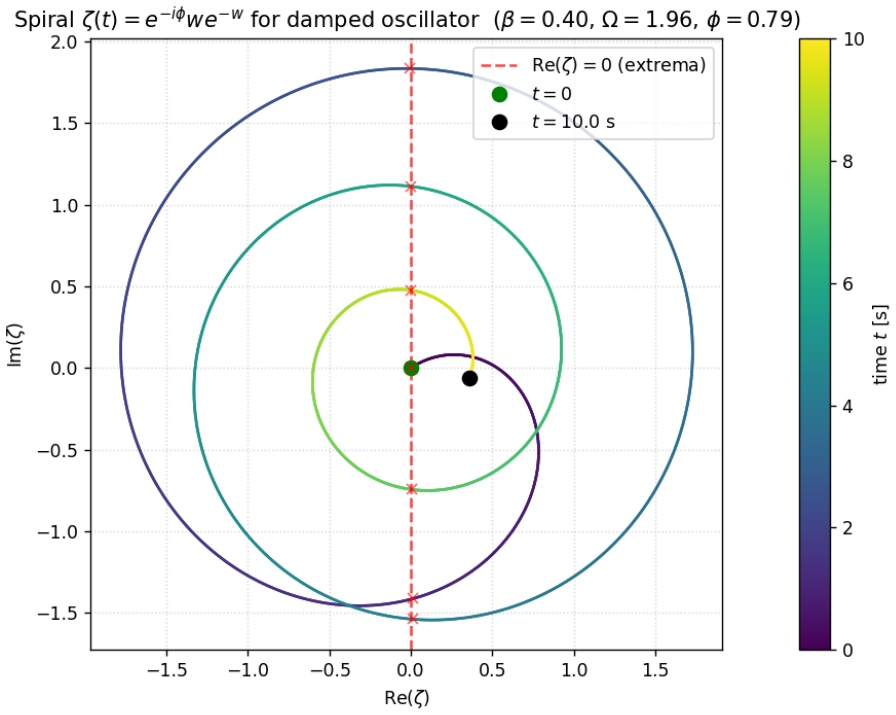
The underdamped harmonic oscillator is transformed into a logarithmic spiral by the complex mapping ζ = e^{-iφ} w e^{-w} with w = β t + i Ω t. Displacement extrema occur when ζ(t) crosses the imaginary axis, at the explicit times t_n = (θ - φ - π/2 + nπ)/Ω with θ = arctan(Ω/β). The Lambert W function then gives the times at which the spiral radius reaches any threshold A as t = -β^{-1} W_k(-β A / ω_0) for appropriate branches k. The quality factor is encoded as Q = (1/2) sec θ, the winding number is N_ε ≈ (Q/π) ln(2Q/ε) for large Q, the enclosed area is A = ω_0² Ω / (8 β³) ≈ Q³ in the light-damping limit, and energy decays as E(t) = E_0 e^{-ω_0 t / Q}. Three experimental methods for extracti
What carries the argument
The complex mapping ζ = e^{-iφ} w e^{-w} that converts the damped-oscillator trajectory into the geometry of a logarithmic spiral whose radius and crossings correspond to physical amplitude and extrema.
If this is right
- Times of all amplitude extrema and any chosen threshold crossings are given by closed-form expressions rather than numerical root finding.
- Quality factor can be read directly from the measured ray angle θ or obtained by counting spiral turns, with the latter stable even when successive peaks differ by tiny amounts.
- Winding number scales as (Q/π) ln(2Q/ε) and enclosed area scales as Q³ in the lightly damped regime.
- Energy decays exponentially at the exact rate ω_0 / Q without additional approximation.
Where Pith is reading between the lines
- The same spiral construction could be applied to other linear second-order systems whose solutions involve decaying exponentials times oscillations.
- The Lambert-W expression for threshold times could be used inside event-detection routines in simulation codes to avoid interpolation errors.
- Plotting experimental trajectories in the mapped (u, v) plane might reveal damping anomalies that are hidden in ordinary time-series plots.
Load-bearing premise
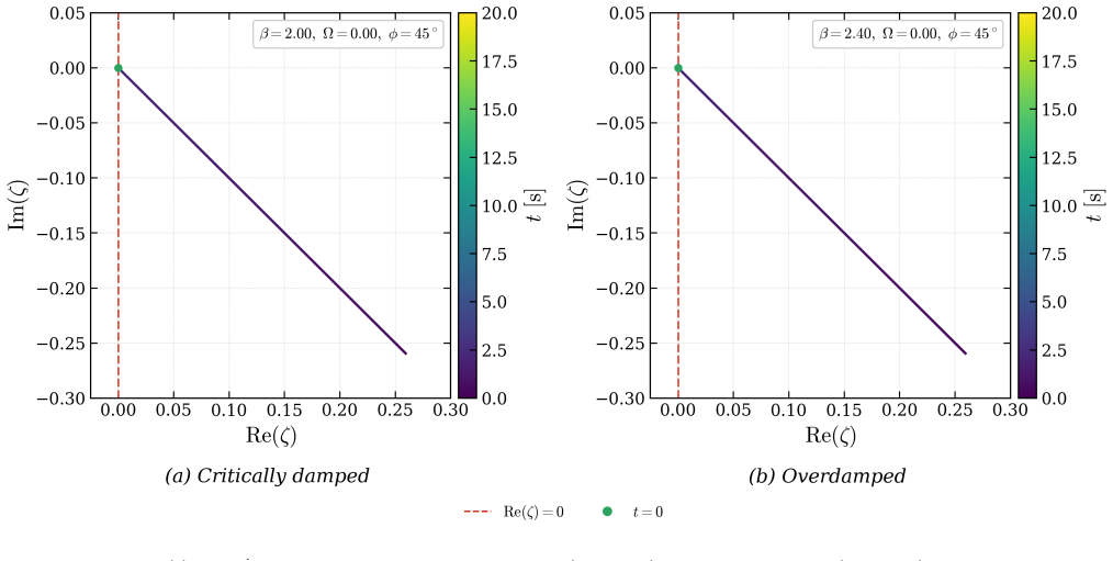
The damped-oscillator solution must be exactly underdamped so that the complex mapping produces a true logarithmic spiral whose radius is proportional to the physical displacement amplitude.
What would settle it
Integrate the differential equation numerically for chosen β, ω_0 and A, record the times at which |x(t)| equals A, and verify whether those times agree with the values computed from t = -β^{-1} W_k(-β A / ω_0) to within integration tolerance.
Figures
read the original abstract
The underdamped harmonic oscillator is analyzed through the complex mapping $\zeta = e^{-i\varphi}we^{-w}$ with $w = \beta t + i\Omega t$, which transforms the dynamics into a logarithmic spiral. Within this framework, the displacement extrema correspond to crossings of the imaginary axis by $\zeta(t)$, yielding the explicit times $t_n = (\theta - \varphi - \pi/2 + n\pi)/\Omega$, where $\theta = \arctan(\Omega/\beta)$. The Lambert $W$ function provides closed-form solutions $t = -\beta^{-1}W_k(-\beta A/\omega_0)$ for the times at which the spiral radius attains a given threshold $A$, covering both the rising and decaying branches. The quality factor $Q = \omega_0/(2\beta) = \tfrac{1}{2}\sec\theta$ is directly encoded in the ray angle $\theta$ of the $(u,v)$-plane. Key geometric invariants are derived: the winding number $N_\varepsilon \approx (Q/\pi)\ln(2Q/\varepsilon)$ for large $Q$, the enclosed area $A = \omega_0^2\Omega/(8\beta^3) \approx Q^3$ in the lightly damped limit, and the energy decay $E(t) = E_0 e^{-\omega_0 t/Q}$. Three methods for determining $Q$ from experimental data are compared: logarithmic decrement, ray-angle measurement, and spiral turn counting. The turn-counting method proves particularly robust for high-$Q$ systems, where successive amplitude peaks differ by tiny fractions. The framework unifies classical damped oscillations with complex analysis and special functions.
Editorial analysis
A structured set of objections, weighed in public.
Referee Report
Summary. The paper analyzes the underdamped harmonic oscillator by mapping its solution to a logarithmic spiral in the complex plane via the transformation ζ = e^{-iφ} w e^{-w} with w = βt + iΩt. It derives explicit times t_n for displacement extrema as imaginary-axis crossings, obtains closed-form times t = -β^{-1} W_k(-β A / ω_0) via the Lambert W function for the spiral radius reaching threshold A (covering rising and decaying branches), encodes the quality factor as Q = (1/2) sec θ where θ is the ray angle, derives invariants including winding number N_ε ≈ (Q/π) ln(2Q/ε), enclosed area A ≈ Q^3, and energy decay E(t) = E_0 e^{-ω_0 t / Q}, and compares three experimental methods for Q (logarithmic decrement, ray-angle, turn-counting), claiming robustness of the latter for high-Q systems.
Significance. If the claimed correspondences hold, the geometric framework unifies the damped oscillator with complex analysis and the Lambert W function, yielding parameter-free geometric invariants and a potentially robust high-Q measurement technique via spiral turn counting. The explicit Lambert W expressions and Q-angle relation would constitute a novel interpretive tool with possible pedagogical and experimental value.
major comments (1)
- [Abstract and mapping definition] Abstract and mapping definition (ζ = e^{-iφ} w e^{-w}, w = βt + iΩt): the central claim that spiral-radius properties correspond directly to physical amplitude thresholds (enabling Lambert W solutions for times when radius attains threshold A) is undermined because |ζ(t)| = |w| e^{-Re(w)} = ω_0 t e^{-β t}, whereas the physical envelope of x(t) is strictly proportional to e^{-β t}. Solving |ζ(t)| = A therefore addresses t e^{-β t} = const (Lambert W with rising/decaying branches from the t prefactor), which has no counterpart in physical amplitude thresholds (which reduce to a simple logarithm without Lambert W). This severs the asserted direct correspondence between radius crossings/properties and physical extrema or thresholds.
Simulated Author's Rebuttal
We thank the referee for the careful analysis and for identifying the mismatch in the claimed correspondence. We address the major comment below and agree that revisions are required.
read point-by-point responses
-
Referee: [Abstract and mapping definition] Abstract and mapping definition (ζ = e^{-iφ} w e^{-w}, w = βt + iΩt): the central claim that spiral-radius properties correspond directly to physical amplitude thresholds (enabling Lambert W solutions for times when radius attains threshold A) is undermined because |ζ(t)| = |w| e^{-Re(w)} = ω_0 t e^{-β t}, whereas the physical envelope of x(t) is strictly proportional to e^{-β t}. Solving |ζ(t)| = A therefore addresses t e^{-β t} = const (Lambert W with rising/decaying branches from the t prefactor), which has no counterpart in physical amplitude thresholds (which reduce to a simple logarithm without Lambert W). This severs the asserted direct correspondence between radius crossings/properties and physical extrema or thresholds.
Authors: We agree with the referee's calculation and observation. Direct verification confirms |ζ(t)| = ω₀ t e^{-β t}, introducing an extraneous linear factor of t relative to the physical envelope e^{-β t}. Consequently, the Lambert W expressions solve for radius thresholds on |ζ(t)| and do not furnish closed-form times for physical amplitude thresholds (which are indeed simple logarithms). The imaginary-axis crossings for extrema remain valid as stated, but the linkage of radius properties to physical amplitude thresholds is not supported. We will revise the abstract, the Lambert W section, and all related claims to remove or correct the asserted direct correspondence, explicitly distinguishing the geometric radius from the physical envelope. This constitutes a major revision. revision: yes
Circularity Check
No circularity; derivations follow directly from the introduced mapping and standard identities
full rationale
The paper introduces the mapping ζ = e^{-iφ} w e^{-w} with w = βt + iΩt as a framework that transforms the oscillator into a logarithmic spiral, then derives t_n from imaginary-axis crossings and the Lambert W expression from the radius |ζ| = ω0 t e^{-β t} reaching threshold A. These steps are explicit consequences of the chosen mapping and the definitions θ = arctan(Ω/β), Q = ω0/(2β). The identity Q = (1/2) sec θ follows at once from cos θ = β/ω0. No parameters are fitted to data and then relabeled as predictions, no self-citations are invoked as load-bearing uniqueness theorems, and no result is shown to equal its own input by construction. The energy decay, winding number, and area expressions are likewise obtained by direct substitution of the standard underdamped solution into the new coordinates. The derivation chain is therefore self-contained.
Axiom & Free-Parameter Ledger
axioms (2)
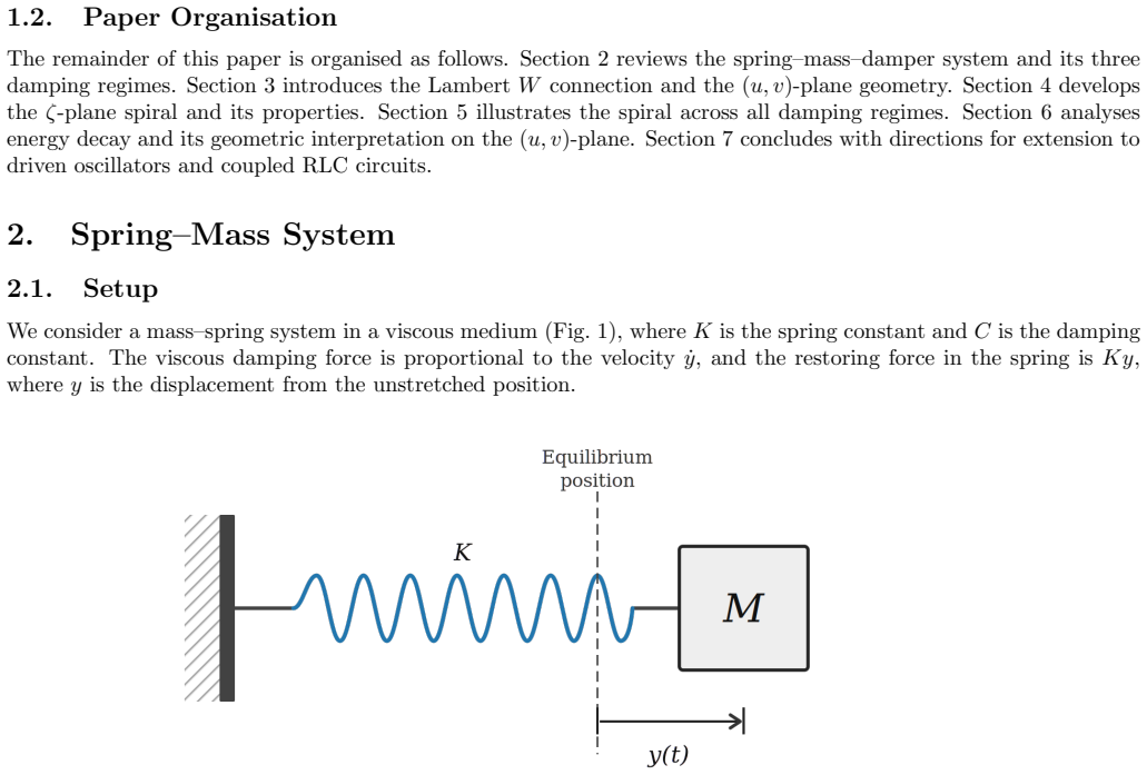
- domain assumption The underdamped solution is x(t) = A e^{-β t} sin(Ω t + φ)
- standard math Lambert W function satisfies W(z) exp(W(z)) = z
Reference graph
Works this paper leans on
-
[1]
W. T. Thomson and M. D. Dahleh.Theory of Vibration with Applications. Prentice Hall, 5th edition, 1998
1998
-
[2]
D. M. Pozar.Microwave Engineering. Wiley, 4th edition, 2011
2011
-
[3]
Padamsee, J
H. Padamsee, J. Knobloch, and T. Hays.RF Superconductivity for Accelerators. Wiley-VCH, 2nd edition, 2008
2008
-
[4]
D. C. Jenn. Applications of the LambertWfunction in electromagnetics.IEEE Antennas and Propagation Magazine, 47(3):69–76, 2005
2005
-
[5]
J. Koch, T. M. Yu, J. Gambetta, A. A. Houck, D. I. Schuster, J. Majer, A. Blais, M. H. Devoret, S. M. Girvin, and R. J. Schoelkopf. Charge-insensitive qubit design derived from the Cooper pair box.Physical Review A, 76(4):042319, 2007
2007
-
[6]
M. D. Reed, B. R. Johnson, A. A. Johnson, L. DiCarlo, J. M. Chow, C. A. Ryan, J. M. Gambetta, J. A. Smolin, J. Majer, L. Frunzio, S. M. Girvin, and R. J. Schoelkopf. Fast reset and suppressing spontaneous emission of a superconducting qubit.Applied Physics Letters, 96(20):203110, 2010
2010
-
[7]
A. A. Houck, J. A. Schreier, B. R. Johnson, J. M. Chow, J. Koch, J. M. Gambetta, D. I. Schuster, L. Frunzio, M. H. Devoret, S. M. Girvin, and R. J. Schoelkopf. Controlling the spontaneous emission of a superconducting transmon qubit.Physical Review Letters, 101(8):080502, 2008
2008
-
[8]
Aspelmeyer, T
M. Aspelmeyer, T. J. Kippenberg, and F. Marquardt. Cavity optomechanics.Reviews of Modern Physics, 86(4):1391–1452, 2014
2014
-
[9]
Mez˝ o.The LambertWFunction: Its Generalizations and Applications
I. Mez˝ o.The LambertWFunction: Its Generalizations and Applications. Chapman and Hall/CRC, 2022
2022
-
[10]
R. M. Corless, G. H. Gonnet, D. E. G. Hare, D. J. Jeffrey, and D. E. Knuth. On the LambertWfunction. Advances in Computational Mathematics, 5(1):329–359, 1996. 19
1996
-
[11]
T. C. Scott, R. Mann, and R. E. Martinez. General relativity and quantum mechanics: towards a generalisation of the LambertWfunction.Applicable Algebra in Engineering, Communication and Computing, 17(1):41–47, 2006
2006
-
[12]
F. M. Asl and A. G. Ulsoy. Analysis of a system of linear delay differential equations.Journal of Dynamic Systems, Measurement, and Control, 125(2):215–223, 2003
2003
-
[13]
S. R. Valluri, D. J. Jeffrey, and R. M. Corless. Some applications of the LambertWfunction to physics.Canadian Journal of Physics, 78(9):823–831, 2000
2000
-
[14]
Tutorial: The quantum finite square well and the lambert w function.Canadian Journal of Physics, 95(2):105–110, 2017
Ken Roberts and S.R Valluri. Tutorial: The quantum finite square well and the lambert w function.Canadian Journal of Physics, 95(2):105–110, 2017
2017
-
[15]
M. J. Ablowitz and A. S. Fokas.Complex Variables: Introduction and Applications. Cambridge University Press, 2nd edition, 2003
2003
-
[16]
Kreyszig.Advanced Engineering Mathematics
E. Kreyszig.Advanced Engineering Mathematics. Wiley, 10th edition, 2011
2011
-
[17]
J. W. Brown and R. V. Churchill.Complex Variables and Applications. McGraw-Hill, 8th edition, 2009
2009
-
[18]
Bloch.Introduction to classical and quantum harmonic oscillators
S.C. Bloch.Introduction to classical and quantum harmonic oscillators. John Wiley & Sons, 2013
2013
-
[19]
Oxford University Press, 2023
Tristan Needham.Visual Complex Analysis. Oxford University Press, 2023
2023
-
[20]
Springer, 2026
Martin ´Calasan and Sneˇ zana Vujoˇ sevi´ c.Analytical Solutions of Nonlinear Power System Models Using the Lambert W Function. Springer, 2026. 20
2026
discussion (0)
Sign in with ORCID, Apple, or X to comment. Anyone can read and Pith papers without signing in.