Balancing Learning Rates Across Layers: Exact Two-Step Dynamics and Optimal Scaling in Linear Neural Networks
Pith reviewed 2026-06-28 23:04 UTC · model grok-4.3
The pith
Test loss in linear neural networks is minimized by unequal learning rates across layers in the first gradient step, with equal rates optimal afterward.
A machine-rendered reading of the paper's core claim, the machinery that carries it, and where it could break.
Core claim
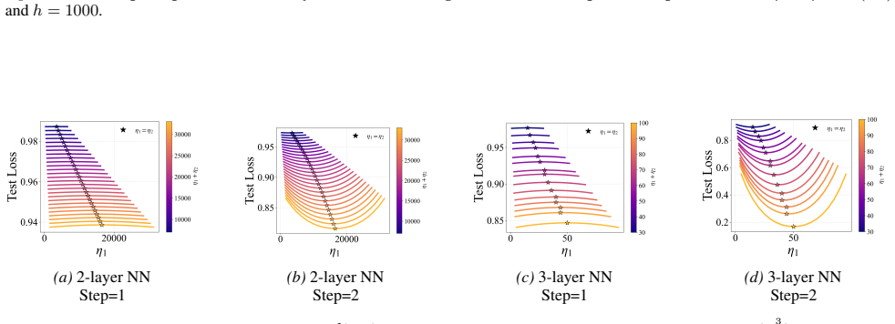
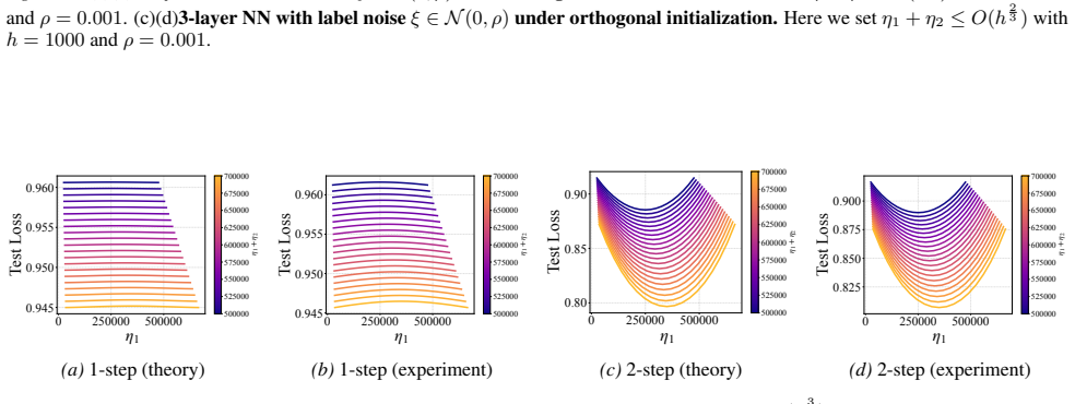
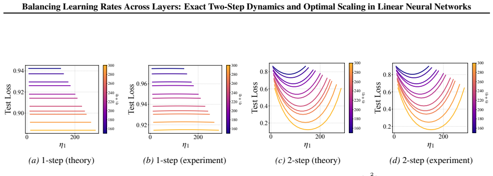
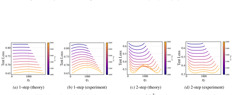
In two- and three-layer linear neural networks trained to learn linear target functions, the exact closed-form expressions for gradients and test loss after one and two steps of gradient descent show that optimal learning rates are unequal across layers at the initial step but equal in subsequent steps. Performing updates with the gradient approximation yields a tractable surrogate loss with a tight, small approximation error, enabling analysis of layer-wise scaling.
What carries the argument
Exact closed-form expressions for the gradients and test loss after one and two steps of gradient descent, which support the characterization of learning-rate scaling under the approximation.
If this is right
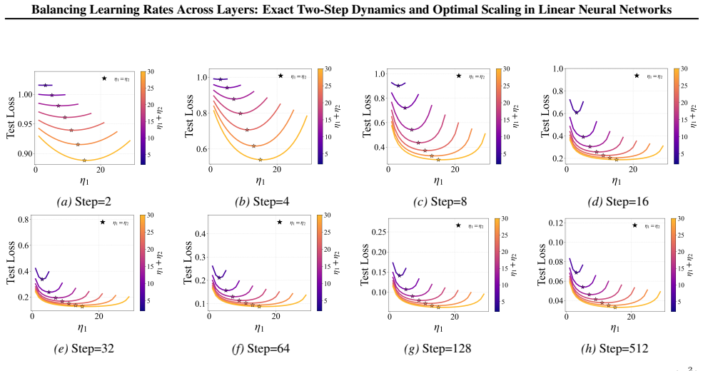
- Unequal learning rates across layers reduce test loss more than equal rates do in the first step.
- Equal learning rates become optimal from the second step onward.
- The surrogate loss approximation has provably small error and supports further theoretical analysis of layer-wise rates.
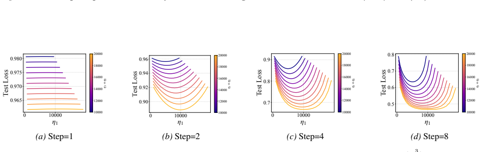
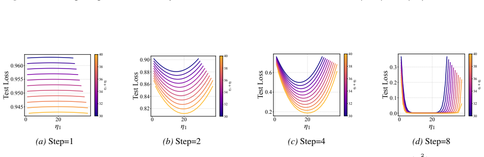
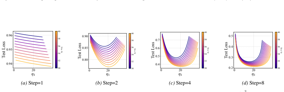
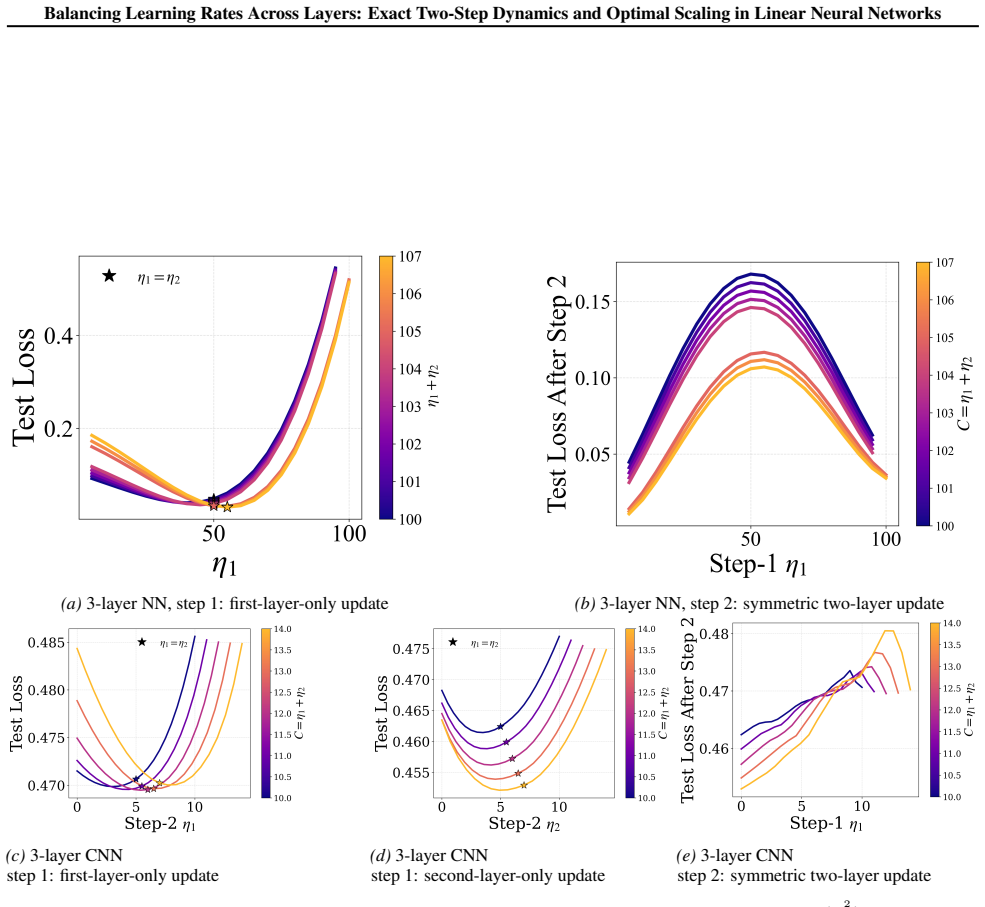
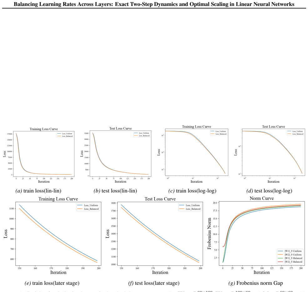
- Numerical experiments on two- and three-layer networks confirm the early-training regime where layer balancing matters.
Where Pith is reading between the lines
- The two-step exact dynamics could be checked for repetition in three or more steps to see if the unequal-to-equal transition pattern persists.
- The initial unequal-rate regime might be tested as a practical heuristic in models that are approximately linear near initialization.
- The surrogate loss construction could be applied to study scaling in wider linear networks without changing the core approximation.
Load-bearing premise
The closed-form derivations and optimality claims hold only for linear networks with linear target functions and are restricted to the first two gradient steps using the gradient approximation.
What would settle it
Training a two-layer linear network on a linear target for two gradient steps and measuring whether the test loss after the first step is lower with unequal per-layer rates than with equal rates would confirm or refute the central claim.
Figures


read the original abstract
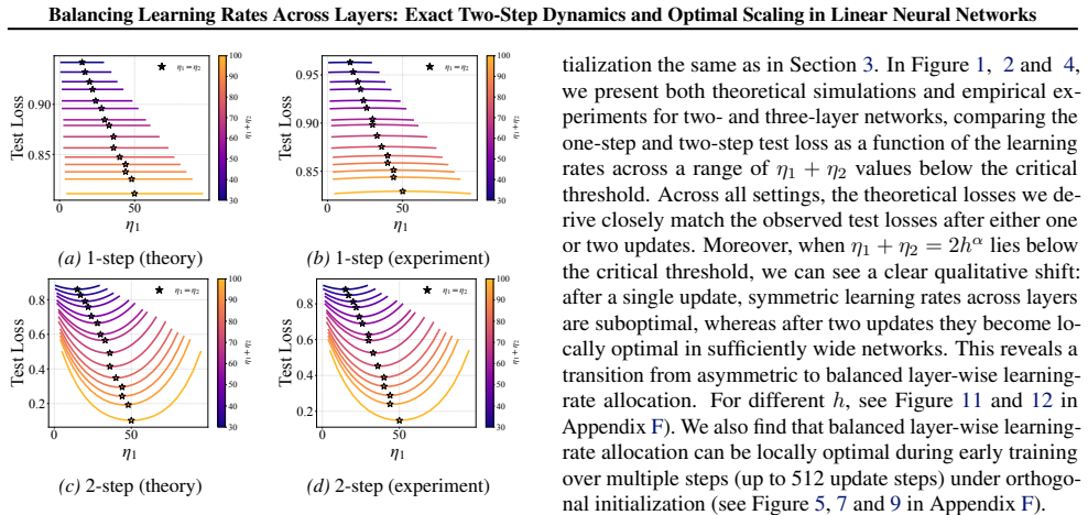
We study optimal learning-rate selection in two-layer and three-layer linear neural networks trained to learn linear target functions. In particular, we derive the exact closed-form expressions for the gradients and test loss after one and two steps of gradient descent, enabling a precise characterization of early training dynamics. We characterize how learning rates should scale under the gradient approximation in the first two steps, and prove that performing updates with this approximation yields a tractable surrogate loss with a tight, small approximation error. This formulation enables the theoretical analysis of layer-wise learning rates and reveals a distinct early-training regime: test loss can be minimized by unequal learning rates at the initial step, while equal learning rates become optimal in subsequent steps. Our numerical experiments validate the theory and demonstrate the importance of balancing layer-wise learning rates early during training. The code is available at: https://github.com/TDCSZ327/Layer-Balancing.
Editorial analysis
A structured set of objections, weighed in public.
Referee Report
Summary. The paper derives exact closed-form expressions for gradients and test loss after one and two steps of gradient descent in two- and three-layer linear neural networks learning linear targets. It characterizes optimal layer-wise learning-rate scaling under a gradient approximation for the first two steps, proves that updates with this approximation yield a tractable surrogate loss with tight small approximation error, and shows that unequal learning rates minimize test loss at the initial step while equal rates become optimal subsequently. Numerical experiments validate the theory; code is provided.
Significance. If the results hold, this supplies precise early-training dynamics for linear networks and highlights the value of unequal layer-wise rates at initialization. The reproducible code and numerical validation are explicit strengths that support the claims.
major comments (2)
- [Abstract] Abstract: the claim that the surrogate loss has a 'tight, small approximation error' underpins the optimality conclusion for unequal rates at step 1, yet no Lipschitz or sensitivity bound is supplied showing that the error does not shift the argmin over the learning-rate vector.
- [Abstract] Abstract: the exact closed-forms and optimality statements are derived only for the first two steps under linear networks and linear targets; the paper provides no argument that the identified early-training regime (unequal then equal rates) survives beyond these restrictions.
Simulated Author's Rebuttal
We thank the referee for the detailed and constructive report. The comments highlight two areas where the abstract claims can be strengthened with additional rigor and clearer scoping. We address each point below and will revise the manuscript accordingly.
read point-by-point responses
-
Referee: [Abstract] Abstract: the claim that the surrogate loss has a 'tight, small approximation error' underpins the optimality conclusion for unequal rates at step 1, yet no Lipschitz or sensitivity bound is supplied showing that the error does not shift the argmin over the learning-rate vector.
Authors: We agree that a formal sensitivity analysis would strengthen the link between the approximation error and the optimality of unequal rates. The current manuscript demonstrates small error numerically and shows that the surrogate preserves the qualitative ordering of test loss, but does not supply an explicit Lipschitz or perturbation bound on the argmin. In the revision we will add a short sensitivity lemma bounding the change in the optimal learning-rate vector as a function of the approximation error, using the fact that the surrogate loss is quadratic in the rates under the linear-network setting. revision: yes
-
Referee: [Abstract] Abstract: the exact closed-forms and optimality statements are derived only for the first two steps under linear networks and linear targets; the paper provides no argument that the identified early-training regime (unequal then equal rates) survives beyond these restrictions.
Authors: The paper deliberately restricts attention to the first two gradient steps in linear networks with linear targets precisely because this regime admits exact closed forms. We do not claim that the unequal-then-equal pattern extends to deeper networks, nonlinear activations, or later training phases; the contribution is the exact characterization and the resulting insight that layer-wise rates should be balanced after the initial step. In the revision we will modify the abstract and introduction to state the scope more explicitly and add a brief paragraph on the limitations and possible extensions. revision: partial
Circularity Check
No significant circularity; derivations are self-contained exact closed forms plus independent error bound
full rationale
The paper derives exact closed-form expressions for gradients and test loss after one and two gradient steps on linear networks, then introduces a gradient approximation to obtain a surrogate loss whose approximation error is separately bounded as tight and small. No step reduces a claimed prediction or optimality result to a fitted parameter by construction, nor does any load-bearing premise rest on a self-citation chain, imported uniqueness theorem, or ansatz smuggled from prior work. The central early-training regime claim follows directly from the closed forms and the stated error bound without circular reduction to inputs.
Axiom & Free-Parameter Ledger
axioms (2)
- standard math Gradient descent follows the standard parameter update rule using the gradient of the loss.
- domain assumption Both the neural network and the target function are linear.
Reference graph
Works this paper leans on
-
[1]
SGDR: Stochastic Gradient Descent with Warm Restarts
PMLR, 2015. Loshchilov, I. and Hutter, F. Sgdr: Stochastic gra- dient descent with warm restarts.arXiv preprint arXiv:1608.03983, 2016. Lu, H., Zhou, Y ., Liu, S., Wang, Z., Mahoney, M. W., and Yang, Y . Alphapruning: Using heavy-tailed self regular- ization theory for improved layer-wise pruning of large language models.Advances in Neural Information Pro...
work page internal anchor Pith review Pith/arXiv arXiv doi:10.1073/pnas.1806579115 2015
-
[2]
= 1√ h (24) A0 2 = A0 2 F = q tr(A0 2 ⊤A0
-
[3]
We have B0 1 = B0 1 F = q tr(B 0 1 ⊤B0
= 1√ h .(25) We also haveB 0 1 = 1 h W 0 1 W 0 2 aa⊤W 0⊤ 2 ,B 0 2 = 1 h W 0⊤ 1 W 0 1 W 0 2 aa⊤ are both rank-1 matrices. We have B0 1 = B0 1 F = q tr(B 0 1 ⊤B0
-
[4]
= 1 h (26) B0 2 = B0 2 F = q tr(B 0 2 ⊤B0
-
[5]
Thus, we get that G0 1 −A 0 1 ≤ 1√ h−1 G0 1 , G0 2 −A 0 2 ≤ 1√ h−1 G0 2
= 1 h .(27) SinceG 0 1 =B 0 1 −A 0 1,G 0 2 =B 0 2 −A 0 2, we obtain that G0 1 −A 0 1 ≤ 1√ h A0 1 ≤ 1√ h ( G0 1 + G0 1 −A 0 1 ) G0 2 −A 0 2 ≤ 1√ h A0 2 ≤ 1√ h ( G0 1 + G0 2 −A 0 2 ). Thus, we get that G0 1 −A 0 1 ≤ 1√ h−1 G0 1 , G0 2 −A 0 2 ≤ 1√ h−1 G0 2 . (28) Based on this, we can get √ h G0 1 = Θh,P(1), √ h G0 1 F = Θh,P(1), √ h G0 2 = Θh,P(1), √ h G0 2...
-
[6]
= 1 h (32) A0 2 = 1 h √ h , A0 2 F = q tr(A0 2 ⊤A0
-
[7]
= 1 h .(33) We also haveB 0 1 = 1 h2 W 0 1 W 0 2 W 0⊤ 2 ,B 0 2 = 1 h W 0⊤ 1 W 0 1 W 0 2 , so we can get that B0 1 = 1 h2 , B0 1 F = q tr(B 0 1 ⊤B0
-
[8]
= 1 h √ h (34) B0 2 = 1 h2 , B0 2 F = q tr(B 0 2 ⊤B0
-
[9]
Thus, we get that G0 1 −A 0 1 ≤ 1√ h−1 G0 1 , G0 2 −A 0 2 ≤ 1√ h−1 G0 2
= 1 h √ h .(35) SinceG 0 1 =B 0 1 −A 0 1,G 0 2 =B 0 2 −A 0 2, we obtain that G0 1 −A 0 1 ≤ 1√ h A0 1 ≤ 1√ h ( G0 1 + G0 1 −A 0 1 ) G0 2 −A 0 2 ≤ 1√ h A0 2 ≤ 1√ h ( G0 1 + G0 2 −A 0 2 ). Thus, we get that G0 1 −A 0 1 ≤ 1√ h−1 G0 1 , G0 2 −A 0 2 ≤ 1√ h−1 G0 2 . (36) Based on this, we can geth √ h G0 1 = Θh,P(1), h G0 1 F = Θh,P(1), h √ h G0 2 = Θh,P(1), h G...
2022
-
[10]
1 h W 1 1 W 1 2 −M ⊤ ˜x⊤ 0 ˜x0 1 h W 1 1 W 1 2 −M #! =tr EW 0 1 ,W 0 2 ,ξ, ˜x0,X
Also consider each row row (or column) of Q is a random vector uniformly distributed on the unit sphere in Rh. Hence by the definitions of orthogonal group, we have hX a=1 Q2 ia = 1⇒E Q2 ia = 1 h , furthermore, if we consider flipping the sign of one row or one column like left-multiplying byD=diag(−1,1,1,· · ·,1) in orthogonal group, which flips the sign...
-
[11]
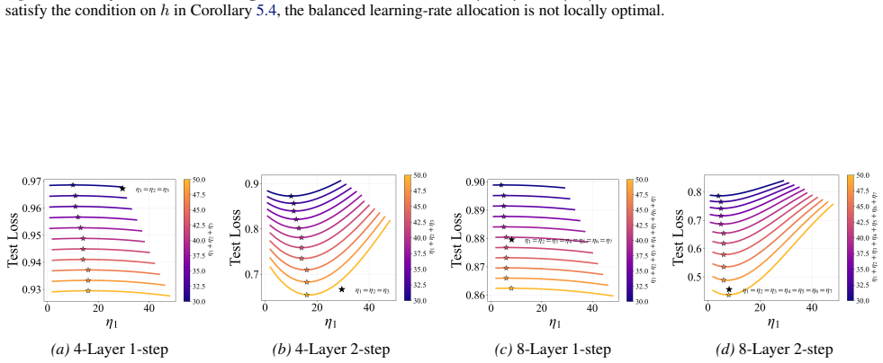
Then, for any α in this range, the point η1 =η 2 =h α is not a local minimum of the lossLtwo-layer(W 1 1 ,W 1 2 ). Moreover, for1< α≤ 3 2, if h >max{h ∗,256} , then η1 =η 2 =h α is a local minimum of the lossL two-layer(W 2 1 ,W 2 2 ), whereh ∗ is the root of the following equation: (1 +o(1))h 1−α + 16hα−2 + 2h−α + 8hα−3 + 6h3α−6 −2 = 0(85) Proof of Corol...
-
[12]
Given the fixed 1< α < 8 5, we will give how large h is to ensure that η1 =η 2 =h α will are local minima, Case 1.Ifα= 3 2, we need 8h 1 2 −32−32−64−o(1)>0, which meansh >256 +o(1). 29 Balancing Learning Rates Across Layers: Exact Two-Step Dynamics and Optimal Scaling in Linear Neural Networks Case 2.If1< α < 3 2, we find6α−13<4α−10<−4and1−α > α−2, so we ...
-
[13]
+η 1η2A0 1(A1 2 −fA1 2)−η 1η2B0 1A1 2 +η 1η2A1 1A1 2 −η 1η2B1 1A1 2 −η 1η2fA1 1 fA1 2 +η 1η2fB1 1 fA1 2 +η 2W 0 1 (B1 2 − fB1
-
[14]
+η 1η2A0 1(B1 2 − fB1
-
[15]
1√ h W 1 1 W 1 2 a−β ∗ ⊤ ˜x⊤ 0 ˜x0 1√ h W 1 1 W 1 2 a−β ∗ # =tr EW 0 1 ,W 0 2 ,a,ξ, ˜x0,X
+η 1η2B0 1B1 2 −η 1η2A1 1B1 2 +η 1η2B1 1B1 2 +η 1η2fA1 1 fB1 2 −η 1η2fB1 1 fB1 2 −η 2W 0 1 B0 2 −η 1η2A0 1B0 2 +η 1η2B0 1B0 2 −η 1η2A1 1B0 2 +η 1η2B1 1B0 2 34 Balancing Learning Rates Across Layers: Exact Two-Step Dynamics and Optimal Scaling in Linear Neural Networks We know that A0 1 ≤O( 1 h √ h ), A0 2 ≤O( 1 h √ h ), B0 1 ≤O( 1 h2 ), B0 2 ≤O( 1 h2 ) gW...
-
[16]
Given the fixed 0< α < 2 3, we will give how large h is to ensure that η1 =η 2 =h α will be the local minima, We need 32h3α−2 + 33hα−1 + 74hα−2 + 2h−α + 10h−α−1 + 36h3α−3 + 4h5α−4 −8<0. □ E. Gaussian Initialization In this section, to obtain more general and practical results, we extend the one-step loss analysis to gaussian initialization while also acco...
2018
-
[17]
1 h W 1 1 W 1 2 −M ⊤ ˜x⊤ 0 ˜x0 1 h W 1 1 W 1 2 −M #! =tr EW 0 1 ,W 0 2 ,ξ, ˜x0,X
Then, for any α in this range, the point η1 =η 2 =h α is not a local minimum of the lossL two-layer(W 1 1 ′ ,W 1 2 ′ ). We do simulations in Figure 6 in Appendix F to support Corollary E.5. E.2.2. THREE-LAYERNEURALNETWORKS Given test data ˜x0 ∼ N(0,I d), we consider the test loss Lthree-layer =E W 0 1 ,W 0 2 ,a,ξ, ˜x0,X 1√ h ˜x0W1W2a− ˜x0β∗ 2 Theorem E.6....
2000
discussion (0)
Sign in with ORCID, Apple, or X to comment. Anyone can read and Pith papers without signing in.