Double-bracket quantum algorithms for thermal state preparation
Pith reviewed 2026-06-28 00:55 UTC · model grok-4.3
The pith
Double-bracket quantum algorithms prepare thermal states by evolving thermofield doubles in imaginary time.
A machine-rendered reading of the paper's core claim, the machinery that carries it, and where it could break.
Core claim
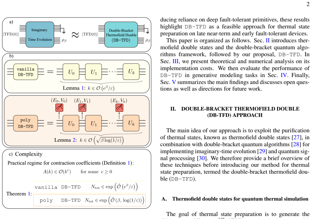
Double-bracket quantum algorithms can implement imaginary-time evolution on thermofield double states so that the reduced state on one subsystem is the target Gibbs thermal state. The poly DB-TFD variant uses double-bracket quantum signal processing to approximate the required evolution operator by a polynomial transformation, producing an algorithm whose complexity grows exponentially with the inverse temperature in a broad practical regime.
What carries the argument
Double-bracket quantum imaginary-time evolution and double-bracket quantum signal processing applied to thermofield double states.
If this is right
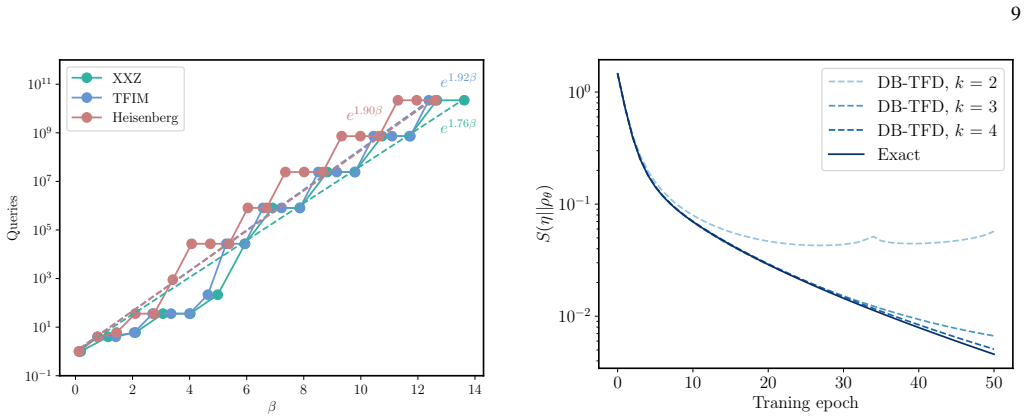
- The complexity of the poly DB-TFD algorithm scales exponentially with the inverse temperature in a broad practical regime.
- Numerical simulations support the theoretical complexity bound for poly DB-TFD.
- DB-TFD improves performance in quantum Boltzmann machines for generative modeling relative to variational imaginary-time evolution.
Where Pith is reading between the lines
- The method may reduce the need for variational optimization when thermal states are required as subroutines in other quantum algorithms.
- If gate costs for the double-bracket primitives stay controlled, the same construction could apply to thermal-state tasks in early fault-tolerant quantum computing.
- Combining thermofield doubles with polynomial approximations might generalize to other non-unitary evolutions beyond imaginary time.
Load-bearing premise
Double-bracket quantum imaginary-time evolution and double-bracket quantum signal processing can be implemented with gate costs that remain practical when applied to thermofield double states whose dimension grows with system size.
What would settle it
A gate-count measurement or numerical simulation on a growing system size showing that the resources needed to realize DB-TFD on thermofield doubles exceed the stated exponential bound in inverse temperature or produce no accuracy gain in quantum Boltzmann machines.
Figures
read the original abstract
We propose quantum algorithms for preparing thermal states via the simulation of the thermofield double states. The key idea is to leverage double-bracket quantum algorithms to implement imaginary-time evolution on thermofield double states, whose reduced state realizes the Gibbs state. Our method, termed double-bracket thermofield double (DB-TFD), introduces two variants. The first, the vanilla DB-TFD algorithm, directly implements imaginary-time evolution using double-bracket quantum imaginary-time evolution. The second, poly DB-TFD, employs double-bracket quantum signal processing to approximate the imaginary-time evolution operator via a polynomial transformation. We demonstrate that the complexity of the poly DB-TFD algorithm scales exponentially with the inverse temperature in a broad practical regime. This scaling is consistent with existing methods, and numerical simulations support the corresponding theoretical bound. We further demonstrate the utility of DB-TFD in quantum Boltzmann machines for generative modeling, achieving improved performance compared with variational imaginary-time evolution approaches. These results establish DB-TFD as a promising route for thermal state preparation in the near-term and early-fault-tolerant regimes.
Editorial analysis
A structured set of objections, weighed in public.
Referee Report
Summary. The manuscript proposes double-bracket thermofield double (DB-TFD) algorithms for thermal state preparation. The vanilla variant directly applies double-bracket quantum imaginary-time evolution to thermofield double states; the poly variant uses double-bracket quantum signal processing to approximate the imaginary-time evolution operator via a polynomial transformation. The central claim is that poly DB-TFD has complexity scaling exponentially with inverse temperature β (consistent with prior methods) in a broad practical regime, with this bound supported by numerical simulations; the method is also shown to improve performance in quantum Boltzmann machines relative to variational imaginary-time evolution.
Significance. If the central claims hold, the work supplies a novel application of double-bracket methods to thermofield-double simulation and thermal-state preparation. The explicit algorithmic constructions and the demonstration of utility for generative modeling via quantum Boltzmann machines are concrete strengths. The claimed exponential-in-β scaling matches the expected information-theoretic cost and would be useful if the implementation costs in the doubled space can be controlled.
major comments (2)
- [poly DB-TFD complexity analysis] The complexity analysis of poly DB-TFD (section describing the algorithm and its scaling): no explicit circuit decomposition or query-complexity bound is supplied for the double-bracket quantum signal processing blocks when applied to thermofield-double states whose Hilbert space dimension scales as 2^{2n}; this assumption is load-bearing for the claim that the exponential-in-β cost remains practical.
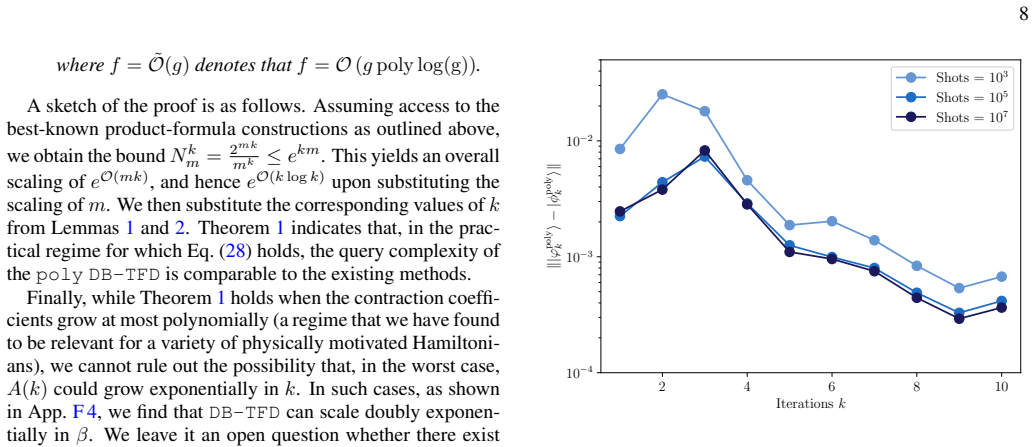
- [numerical results] Numerical simulations supporting the exponential scaling bound (results section): the manuscript states that numerics corroborate the theoretical bound, yet provides neither error bars, dataset sizes, number of independent runs, nor explicit circuit constructions; demonstrations are confined to small instances where the doubled-space overhead is invisible, undermining verification of the central complexity claim.
minor comments (2)
- [introduction] Notation for the thermofield-double state and its reduced density matrix could be introduced more explicitly in the opening sections to aid readers unfamiliar with the doubled-space construction.
- [results] A short table comparing gate counts or query complexities of DB-TFD variants against standard methods (e.g., variational imaginary-time evolution) would improve clarity of the claimed advantages.
Simulated Author's Rebuttal
We thank the referee for their thorough review and valuable comments on our manuscript. We address each major comment below and plan to revise the manuscript to incorporate the suggested improvements.
read point-by-point responses
-
Referee: [poly DB-TFD complexity analysis] The complexity analysis of poly DB-TFD (section describing the algorithm and its scaling): no explicit circuit decomposition or query-complexity bound is supplied for the double-bracket quantum signal processing blocks when applied to thermofield-double states whose Hilbert space dimension scales as 2^{2n}; this assumption is load-bearing for the claim that the exponential-in-β cost remains practical.
Authors: We agree that providing an explicit query complexity bound would strengthen the manuscript. The poly DB-TFD complexity is derived by composing the known bounds for double-bracket quantum signal processing (which approximate the imaginary-time evolution with polynomial degree scaling exponentially in β) with the thermofield double construction. The Hilbert space dimension 2^{2n} affects the cost of implementing the Hamiltonian oracle but does not alter the exponential-in-β scaling. In the revised version, we will include a dedicated paragraph or subsection with the explicit bound, expressed in terms of queries to the doubled-space Hamiltonian. revision: yes
-
Referee: [numerical results] Numerical simulations supporting the exponential scaling bound (results section): the manuscript states that numerics corroborate the theoretical bound, yet provides neither error bars, dataset sizes, number of independent runs, nor explicit circuit constructions; demonstrations are confined to small instances where the doubled-space overhead is invisible, undermining verification of the central complexity claim.
Authors: We will enhance the numerical results section in the revision by adding error bars, specifying the number of independent runs (we used 50 runs per data point), and detailing the dataset sizes. We will also provide more details on the circuit constructions used in the simulations, such as the number of gates for the double-bracket steps. While the simulations are performed on small systems to demonstrate the principle and scaling trend, the theoretical analysis explicitly accounts for the doubled space dimension. We believe these additions will allow better verification of the claims. revision: yes
Circularity Check
No significant circularity: scaling bound derived independently and supported by numerics
full rationale
The abstract presents the exponential-in-β complexity of poly DB-TFD as a derived theoretical bound that is merely shown to be consistent with prior methods and corroborated by numerical simulations on small instances. No equation or claim reduces the scaling to a fitted parameter, self-defined quantity, or load-bearing self-citation chain; the derivation chain remains self-contained against external benchmarks and does not exhibit any of the enumerated circularity patterns.
Axiom & Free-Parameter Ledger
axioms (1)
- domain assumption Double-bracket quantum imaginary-time evolution and double-bracket quantum signal processing can be realized with gate costs polynomial in system size for the relevant thermofield double Hamiltonians.
Reference graph
Works this paper leans on
-
[1]
Double-bracket quantum imaginary-time evolution (DB-QITE) This section summarizes results from Ref. [29], which show that imaginary-time evolution is a solution to the double-bracket flow and introduce a quantum algorithm termed the Double-Bracket Quantum Imaginary-Time Evolution (DB-QITE) algorithm. Imaginary-time evolution is defined as |Φ(τ)⟩ = e−τ H|Φ...
-
[2]
[30], which proposes a quantum algorithm for constructing matrix-valued polyno- mial functions without the use of ancilla qubits or post-selection
Double-bracket quantum signal processing (DB-QSP) This section summarizes results from Ref. [30], which proposes a quantum algorithm for constructing matrix-valued polyno- mial functions without the use of ancilla qubits or post-selection. The approach relies on double-bracket quantum algorithms and is referred to as Double-Bracket Quantum Signal Processi...
-
[3]
kX i Yi > l # = 2PY
Approximating a monomial using Chebyshev polynomials We first show that a monomial xk can be approximated using a polynomial pk,l(x) of degree l ∈ O( √ k) over the interval [−1, 1]. This analysis focuses on a uniform approximation, and therefore on bounding sup x∈[−1,1] |xk − pk,l(x)|. (D3) Let Y be a random binary variable taking the value 1 and−1 with e...
-
[4]
Approximating exponential functions using Chebyshev polynomials We now approximate exp(−x) via polynomials of order O(√β) on the interval x ∈ [0, β]. Specifically, we approximate the Taylor series of the exponential using the monomial approximation outlined above, which can reduce the required polynomial degree from O(β) to O(√β). First, the interval of a...
-
[5]
To this end, we first quantify the error introduced by the approximation
Vanilla DB approach: Proof of Lemma 1 We show the number of steps k required for the vanilla DB-TFD state |ψ(vanilla) k ⟩, corresponding to a perfect imple- mentation of the exponential of the commutator, to approximate the thermofield double state at inverse temperature β/2 with ε-precision. To this end, we first quantify the error introduced by the appr...
-
[6]
The first term can be directly bounded as |ψ(vanilla) j+1 ⟩ − es[ψ(vanilla) j ,H]|ψ(ITE) j ⟩ = es[ψ(vanilla) j ,H]|ψ(vanilla) j ⟩ − es[ψ(vanilla) j ,H]|ψ(ITE) j ⟩ ≤ es[ψ(vanilla) j ,H] op |ψ(vanilla) j ⟩ − |ψ(ITE) j ⟩ = ∆j, (E5) where we use the unitarity of the exponential of the commutator, implying ∥es[ψ(vanilla) j ,H]∥op = 1
-
[7]
As for the second term, we obtain es[ψ(vanilla) j ,H]|ψ(ITE) j ⟩ − es[ψ(ITE) j ,H]|ψ(ITE) j ⟩ ≤ es[ψ(vanilla) j ,H] − es[ψ(ITE) j ,H] op |ψ(ITE) j ⟩ = es[ψ(vanilla) j ,H] − es[ψ(ITE) j ,H] op , (E6) where ∥|ψ(ITE) j ⟩∥ = 1. Since ∥eA − eB∥op ≤ ∥A − B∥op, (E7) in case eA and eB are unitaries, we get es[ψ(vanilla) j ,H] − es[ψ(ITE) j ,H] op ≤ s[ψ(vanilla) j...
-
[8]
To simplify the last term, we exploit the Lagrange remainder theorem for both operations; namely, we have the expressions es[ψ(ITE) j ,H]|ψ(ITE) j ⟩ = (1 + ∂ses[ψ(ITE) j ,H]|s=0 + RDB)|ψ(ITE) j ⟩, (E9) and |ψ(ITE) j+1 ⟩ = e−sH |ψ(ITE) j ⟩ e−sH |ψ(ITE) j ⟩ = 1 + ∂s e−sH e−sH |ψ(ITE) j ⟩ s=0 + RITE |ψ(ITE) j ⟩. (E10) The first-order derivativ...
-
[9]
Similar to the case for vanilla DB-TFD, we first estimate the error incurred by the approximation
Poly DB approach: Proof of Lemma 2 We show the polynomial degree k required for the poly DB-TFD state |ψ(poly) k ⟩, corresponding to a perfect implementation of the exponential of the commutator, to approximate the thermofield double state at inverse temperature β/2 with ε-precision. Similar to the case for vanilla DB-TFD, we first estimate the error incu...
-
[10]
Define two sequences of states
Proof of Lemma 3 We bound the error between the exact implementation of the exponential of commutators and its approximation obtained from an order-m product formula over multiple iterations. Define two sequences of states. The first corresponds to the exact implementation of the exponential of the commutator, |ψ(vanilla) j+1 ⟩ = jY i=0 esi[ψ(vanilla) i ,...
-
[11]
We introduce an upper bound for the first two terms as ∥ |ψ(vanilla) j+1 ⟩ − esj[ψ(vanilla) j ,H] |ϕ(vanilla) j ⟩ ∥ + ∥esj[ψ(vanilla) j ,H] |ϕ(vanilla) j ⟩ − esj[ϕ(vanilla) j ,H] |ϕ(vanilla) j ⟩ = aj∆j, (F5) where aj ≥ 0 characterizes the effective contraction
-
[12]
That is, we have ∥esj[ϕ(vanilla) j ,H] − U(vanilla) PF,j ∥op ≤ Cs m+1 2 j
For the third term, we start with the simplification; ∥esj[ϕ(vanilla) j ,H] |ϕ(vanilla) j ⟩−|ϕ(vanilla) j+1 ⟩ ∥ ≤ ∥ esj[ϕ(vanilla) j ,H]−U(vanilla) PF,j ∥op∥ |ϕ(vanilla) j ⟩ ∥ = ∥esj[ϕ(vanilla) j ,H]−U(vanilla) PF,j ∥op, (F6) which allows us to straightforwardly use the error bound for product-formula approximation. That is, we have ∥esj[ϕ(vanilla) j ,H] ...
-
[13]
(F13) For clarity, we assume throughout that the operator norm of the Hamiltonian satisfies ∥H∥op ≤ 1
Setting product formula order We now determine the order of the product formula required to achieve the error bound: |ψ(vanilla) k ⟩ − |ϕ(vanilla) k ⟩ ≤ ε. (F13) For clarity, we assume throughout that the operator norm of the Hamiltonian satisfies ∥H∥op ≤ 1. Before proceeding, we specify the constant C appearing in the error bound. This constant originate...
-
[14]
Setting product formula order using the general bound on contraction coefficient Lemma F.5(Error incurred by anm-th order product formula). Let U(v) DB,k denote the k-step DB-TFD using the exact exponential of the commutators, and let U(v) P F,k denote the corresponding unitary using an m-th order product formula with Nm factors, for v = {vanilla, poly}. ...
-
[15]
The first term can be bounded as ∥ |ψ(vanilla) j+1 ⟩ − esj[ψ(vanilla) j ,H] |ϕ(vanilla) j ⟩ ∥ ≤ ∥ esj[ψ(vanilla) j ,H] |ψ(vanilla) j ⟩ − esj[ψ(vanilla) j ,H] |ϕ(vanilla) j ⟩ ∥ ≤ ∥esj[ψ(vanilla) j ,H]∥op∥ |ψ(vanilla) j ⟩ − |ϕ(vanilla) j ⟩ ∥ = ∆j, (F29) where we use the fact that the norm of a unitary is one in the last equality
-
[16]
(F30) In the second inequality we use ∥ |ϕ(vanilla) j ⟩ ∥ = 1
The second term is first simplified as ∥esj[ψ(vanilla) j ,H] |ϕ(vanilla) j ⟩ − esj[ϕ(vanilla) j ,H] |ϕ(vanilla) j ⟩ ∥ ≤ ∥ esj[ψ(vanilla) j ,H] − esj[ϕ(vanilla) j ,H]∥op∥ |ϕ(vanilla) j ⟩ ∥ ≤ ∥esj[ψ(vanilla) j ,H] − esj[ϕ(vanilla) j ,H]∥op. (F30) In the second inequality we use ∥ |ϕ(vanilla) j ⟩ ∥ = 1. Since ∥eA − eB∥op ≤ ∥A − B∥op, (F31) in case eA and eB ...
-
[17]
That is, we have ∥esj[ϕ(vanilla) j ,H] − U(vanilla) PF,j ∥op ≤ Cs m+1 2 j
For the third term, we start with the simplification; ∥esj[ϕ(vanilla) j ,H] |ϕ(vanilla) j ⟩−|ϕ(vanilla) j+1 ⟩ ∥ ≤ ∥ esj[ϕ(vanilla) j ,H]−U(vanilla) PF,j ∥op∥ |ϕ(vanilla) j ⟩ ∥ = ∥esj[ϕ(vanilla) j ,H]−U(vanilla) PF,j ∥op, (F33) which allows us to straightforwardly use the error bound for product-formula approximation. That is, we have ∥esj[ϕ(vanilla) j ,H]...
-
[18]
Theorem F.2 (Oracle calls to Hamiltonian evolutions and reflection operators required to prepare |TFD(β)⟩ within error-preci- sion ε)
Lower bound on the total number of operations We finally assess the total number of operations required to achieve ε-precision in implementing the exact commutators using the product formula of order m. Theorem F.2 (Oracle calls to Hamiltonian evolutions and reflection operators required to prepare |TFD(β)⟩ within error-preci- sion ε). To achieve an ε-pre...
-
[19]
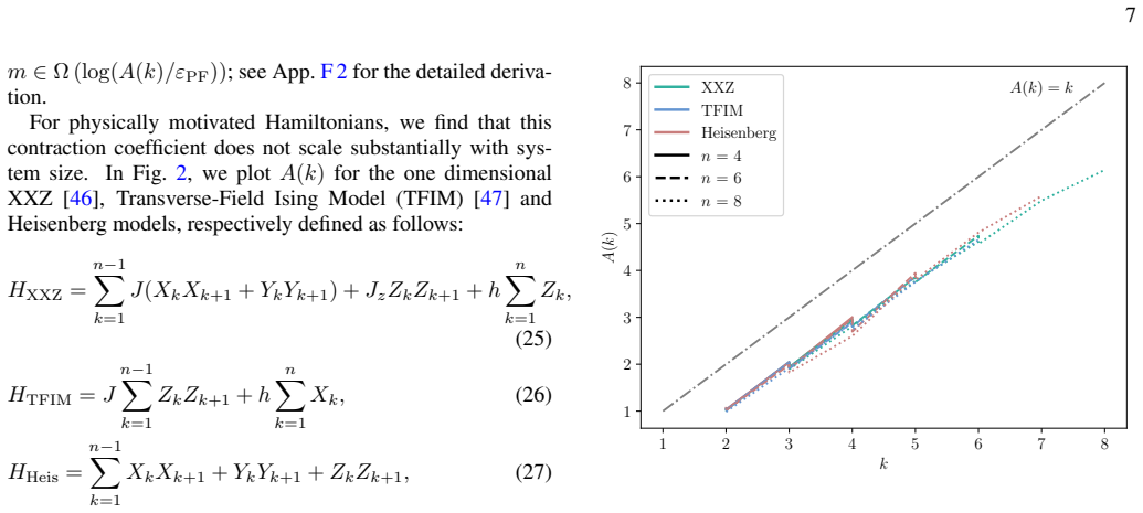
(28), we assume that the contraction coefficient can be bounded by a polynomial in k as follows: A(k) = k−1X i=1 kY j=i aj ∈ O(kc) (F50) for some constant c ≥ 0
Proof of Lemma 4 Using Lemma 3, as stated in Eq. (28), we assume that the contraction coefficient can be bounded by a polynomial in k as follows: A(k) = k−1X i=1 kY j=i aj ∈ O(kc) (F50) for some constant c ≥ 0. Thus, the total error accumulation is bounded strictly by a polynomial bound: ∆k ≤ O kc Cs m+1 2 max . (F51)
-
[20]
From App
Setting product formula order in the practical regime We determine the product formula order m to satisfy the error bound ∆k ≤ ε. From App. F 2, the constant C appearing in the error bound is given by C ≤ α2m+1 (m + 1)!. (F52) Using the bound derived in Eq. (F51), and introducing γ as the constant factor from the O(kc) bound, we require the total accumula...
-
[21]
From App
Lower bound on the total number of operations for efficient cases We finally assess the total number of operations required to achieve ϵ-precision in implementing the exact commutators using the product formula of order m. From App. F 4, the total query complexity scales as eO(km). Then, using the product formula order found in App. F 6, we have ekm ≥ e2e...
-
[22]
As shown in App
Error propagation in parameters due to statistical noise In this section, we analyze the error propagation of the statistical noise for parameters s and θ in poly DB-TFD. As shown in App. C 2, each iteration step j requires the estimation of sj = − 1p Vj arccos |Ej − z|p Vj + |Ej − z|2 ! (F60) θj = arg Ej − z |Ej − z| , (F61) where Ej and Vj are the energ...
-
[23]
Bounding the first term: First, we need to compute the partial derivative of s(V, d) with respect to V . Defining u = √ V d for simplicity, we obtain ∂s(V, d) ∂V = − 1 2V 3/2 arctan(u) + 1√ V 1 1 + u2 1 2d √ V = − 1 2V 3/2 arctan(u) + 1 2V (d2 + V ) d = − 1 2V 3/2 arctan(u) − d √ V d2 + V ! = − 1 2V 3/2 arctan(u) − u 1 + u2 (F71) 39 Since arctan(u) ≥ u 1+...
-
[24]
Bounding the second term: Similar to the first term, we start with computing the partial derivative ofs(V, d) with respect to d and obtain ∂s(V, d) ∂d = 1√ V 1 1 + ( √ V /d)2 − √ V d2 ! = − 1 V + d2 . (F77) By the Mean Value Theorem, there exists some intermediate d∗ j between dj and ˆdj, such that |s( ˆVj, dj) − s( ˆVj, ˆdj)| ≤ ∂s(V, d) ∂d ( ˆVj ,d∗ j ) ...
-
[25]
Since the vanilla approach requires no intermediate measurements, we only study this error for the poly DB-TFD
Error due to the statistical noise Here, we bound the error incurred by replacing the exact energies and variances appearing in anm-order product formula with their estimated values. Since the vanilla approach requires no intermediate measurements, we only study this error for the poly DB-TFD. For the poly DB-TFD , the parameters {(θi, si)} depend explici...
-
[26]
For the first term, we obtain ∥U j θ U j s |ϕ(poly) j ⟩ − U j θ U j s |φ(poly) j ⟩∥ = ∥U j θ U j s |ϕ(poly) j ⟩ − |φ(poly) j ⟩ ∥ = ∥|ϕ(poly) j ⟩ − |φ(poly) j ⟩∥ = ˆ∆j, (F98) where we use the unitary invariance in the second line
-
[27]
Moreover, in the last line, we use ∥ϕ(poly) j − φpoly j ∥op ≤ 2∥|ϕ(poly) j ⟩ − |φpoly j ⟩∥
For the second term, we have ∥U j θ U j s |φ(poly) j ⟩ − ˆU j θ U j s |φ(poly) j ⟩∥ = ∥ U j θ − ˆU j θ U j s |φ(poly) j ⟩∥ ≤ ∥U j θ − ˆU j θ ∥op · ∥U j s |φ(poly) j ⟩∥ ≤ ∥U j θ − ˆU j θ ∥op = ∥eiθj ϕ(poly) j − eiθj φ(poly) j ∥op ≤ |θj| ∥ϕ(poly) j − φ(poly) j ∥op ≤ 2|θj| ∥|ϕ(poly) j ⟩ − |φ(poly) j ⟩∥ = 2|θj| ˆ∆j, (F99) where we use the fact that ∥AB∥ ≤ ∥ A...
-
[28]
Moreover, using the definition of the operators in Eq
The third term is give by ∥ ˆU j θ U j s |φ(poly) j ⟩ − ˆU j θ ˆU j s |φ(poly) j ⟩∥ = ∥ ˆU j θ U j s − ˆU j s |φ(poly) j ⟩∥ ≤ ∥ ˆU j θ ∥op ∥U j s − ˆU j s ∥op ≤ ∥U j s − ˆU j s ∥op, (F100) 42 where we use a normalised state assumption and the property ∥AB∥ ≤ ∥ A∥ ∥B∥ in the second line. Moreover, using the definition of the operators in Eq. (F93) and Eq. ...
-
[29]
For the fourth term, similar to the second term, we have ∥ ˆU j θ ˆU j s |φ(poly) j ⟩ − ˆU j ˆθ ˆU j s |φ(poly) j ⟩∥ ≤ ∥ ˆU j θ − ˆU j ˆθ ∥op. (F104) Then since ˆU j θ = eiθj φ(poly) j and ˆU j ˆθ = eiˆθj φ(poly) j , using the fact that φ(poly) j is a pure state, we have ∥ ˆU j θ − ˆU j ˆθ ∥op = ∥ 1 + (eiθj − 1)φ(poly) j − 1 + (eiˆθj − 1)φ(poly) j ∥op (F1...
-
[30]
(F108) 43 Then, we can upper bound ∥ ˆU j s − ˆU j ˆs ∥ similar to the third term
Finally, for the fifth term, we have ∥ ˆU j ˆθ ˆU j s |φ(poly) j ⟩ − ˆU j ˆθ ˆU j ˆs |φ(poly) j ⟩∥ = ∥ ˆU j ˆθ ˆU j s − ˆU j ˆs |φ(poly) j ⟩∥ ≤ ∥ ˆU j s − ˆU j ˆs ∥op. (F108) 43 Then, we can upper bound ∥ ˆU j s − ˆU j ˆs ∥ similar to the third term. According to Eq. (F94) and Eq. (F95), we have ∥ ˆU j s − ˆU j ˆs ∥op = ∥eiα1 √sj H eiα2 √sj φ(poly) j · · ...
-
[31]
Numerical implementation of DB-TFD with exponential of exact commutators Both the vanilla DB-TFD and the poly DB-TFD require the exponential of commutators, and hence we first elaborate on their numerical implementation. To implement the exponential of commutators, we utilize the Python package SciPy [78], taking advantage of its sparse matrix functionali...
-
[32]
(G1) reads es[ψ,H]|ψ⟩ = cos(s √ V )|ψ⟩ − sin(s √ V )√ V |v⟩
|v⟩ = |h⟩ − E|ψ⟩ Then, the exponential of the commutator in Eq. (G1) reads es[ψ,H]|ψ⟩ = cos(s √ V )|ψ⟩ − sin(s √ V )√ V |v⟩. (G2) Thus, this computation requires only a single matrix-vector multiplication and two inner products. For the poly DB-TFD approach, the roots of the polynomial are required to factorize it and determine the corresponding time step...
-
[33]
= es2[A,B] + O(xm+1), (G7) where tk = αks with a specific coefficient αk
Numerical implementation of the product-formula approximation An m-th order product-formula approximation of the exponential of commutators is given by es2[A,B] = et1Aet2Bet3Aet4B... = es2[A,B] + O(xm+1), (G7) where tk = αks with a specific coefficient αk. Explicit formulas for second- and third-order product formulas, as well as recursive constructions f...
-
[34]
First, we briefly review quantum generative modeling using quantum Boltzmann machines
Numerical setting for generative modeling tasks We provide the details of the numerical setups used for generative modeling tasks in the main text. First, we briefly review quantum generative modeling using quantum Boltzmann machines. Next, we describe the specific tasks considered in this study, followed by a short overview of Variational Quantum Imagina...
discussion (0)
Sign in with ORCID, Apple, or X to comment. Anyone can read and Pith papers without signing in.