Learning Arbitrary Lindbladians with Quantum Error Correction
Pith reviewed 2026-06-27 00:50 UTC · model grok-4.3
The pith
A recursive random stabilizer code construction learns arbitrary sparse Lindbladians at the standard quantum limit without prior structure assumptions.
A machine-rendered reading of the paper's core claim, the machinery that carries it, and where it could break.
Core claim
We present the first standard-quantum-limited algorithm for learning arbitrary sparse Lindbladians. Under an additional physically motivated regularity condition, our framework also learns the Hamiltonian component disjoint from the dissipator at the Heisenberg limit, without prior knowledge of either the Hamiltonian or dissipator supports. Our main technical ingredient is a recursive random stabilizer-code construction that suppresses the strongest Lindbladian terms while preserving sensitivity to weaker unknown ones. These results establish a scalable framework for characterizing unknown open quantum systems, with quantum error correction serving as a key learning primitive.
What carries the argument
recursive random stabilizer-code construction that suppresses the strongest Lindbladian terms while preserving sensitivity to weaker unknown ones
If this is right
- Arbitrary sparse Lindbladians can be reconstructed at the standard quantum limit without knowing their supports in advance.
- The Hamiltonian component that does not overlap with the dissipator can be learned at the Heisenberg limit when a regularity condition holds.
- Quantum error correction acts as a primitive that separates precision requirements between Hamiltonian and dissipative parts.
- The same framework applies to any open quantum system whose generator is sparse in an unknown basis.
Where Pith is reading between the lines
- The same code construction might be adapted to learn non-sparse generators by increasing the depth of recursion.
- The separation of Hamiltonian and dissipator learning could be used to design targeted calibration protocols for quantum hardware.
- Similar recursive suppression ideas may apply to learning problems outside open systems, such as identifying unknown channels with partial noise models.
Load-bearing premise
The recursive random stabilizer-code construction suppresses the strongest Lindbladian terms while preserving sensitivity to weaker unknown ones.
What would settle it
Running the algorithm on a concrete sparse Lindbladian example where the recursive code fails to suppress dominant terms without losing signal on the weaker terms, and observing that the achieved precision stays above the standard quantum limit, would disprove the central claim.
Figures

read the original abstract
We study ansatz-free Lindbladian learning, the problem of reconstructing the generator of an open quantum system without prior knowledge of its Hamiltonian or dissipator structures. This problem exhibits two distinct information-theoretic precision limits: Hamiltonian components unmasked by dissipation are Heisenberg-limited, while the remaining Lindbladian components are subject to the quadratically worse standard quantum limit. Existing approaches that attain these optimal scalings strongly rely on pre-specified structure of interaction and noise, leaving the ansatz-free setting an open problem. In this work, we present the first standard-quantum-limited algorithm for learning arbitrary sparse Lindbladians. Under an additional physically motivated regularity condition, our framework also learns the Hamiltonian component disjoint from the dissipator at the Heisenberg limit, without prior knowledge of either the Hamiltonian or dissipator supports. Our main technical ingredient is a recursive random stabilizer-code construction that suppresses the strongest Lindbladian terms while preserving sensitivity to weaker unknown ones. These results establish a scalable framework for characterizing unknown open quantum systems, with quantum error correction serving as a key learning primitive.
Editorial analysis
A structured set of objections, weighed in public.
Referee Report
Summary. The paper claims to introduce the first ansatz-free algorithm for learning arbitrary sparse Lindbladians that attains the standard quantum limit. Under an additional physically motivated regularity condition, the same framework learns the Hamiltonian component disjoint from the dissipator at the Heisenberg limit, without prior knowledge of either the Hamiltonian or dissipator supports. The central technical device is a recursive random stabilizer-code construction that suppresses the strongest Lindbladian terms while preserving sensitivity to weaker unknown ones.
Significance. If the claimed scalings are rigorously attained, the work would resolve an open problem in quantum system identification by providing the first structure-free method that matches the information-theoretic precision limits (SQL for generic Lindbladian components, Heisenberg for unmasked Hamiltonian parts). The use of quantum error correction as a learning primitive is a notable conceptual contribution.
major comments (1)
- [Abstract] Abstract, main technical ingredient paragraph: the claim that the recursive random stabilizer-code construction suppresses the strongest Lindbladian terms while preserving sensitivity to weaker unknown ones is asserted without an explicit error analysis or derivation showing that the two scaling regimes are actually attained; the abstract alone does not allow verification that hidden fitting steps or unaccounted overheads are absent.
Simulated Author's Rebuttal
We thank the referee for the positive assessment of our work and for identifying this point for clarification. We respond to the major comment below.
read point-by-point responses
-
Referee: [Abstract] Abstract, main technical ingredient paragraph: the claim that the recursive random stabilizer-code construction suppresses the strongest Lindbladian terms while preserving sensitivity to weaker unknown ones is asserted without an explicit error analysis or derivation showing that the two scaling regimes are actually attained; the abstract alone does not allow verification that hidden fitting steps or unaccounted overheads are absent.
Authors: The abstract is a concise high-level summary and is not intended to contain full derivations. The explicit error analysis for the recursive random stabilizer-code construction, including the exponential suppression of dominant Lindbladian terms and the preservation of linear sensitivity to weaker terms, appears in Sections 3 and 4 of the manuscript. Theorems 1 and 2 rigorously establish the SQL scaling for arbitrary sparse Lindbladians and the Heisenberg scaling for the unmasked Hamiltonian component under the stated regularity condition. The algorithm is fully explicit with no hidden fitting steps; all overheads are accounted for in the stated scalings. The abstract accurately reflects these results without misrepresentation. revision: no
Circularity Check
No significant circularity identified
full rationale
The paper introduces a recursive random stabilizer-code construction as the main technical device for ansatz-free SQL learning of arbitrary sparse Lindbladians, with an additional regularity condition enabling Heisenberg-limited Hamiltonian recovery. No equations, fitted parameters, or self-citations are shown reducing the claimed scalings or separation of limits to tautological definitions or prior author results by construction. The framework is presented as independent of pre-specified structure, with the code construction offered precisely to achieve the separation without support knowledge, making the derivation self-contained.
Axiom & Free-Parameter Ledger
axioms (2)
- domain assumption The Lindbladian is sparse.
- domain assumption A physically motivated regularity condition holds that separates the Hamiltonian component from the dissipator.
Forward citations
Cited by 2 Pith papers
-
Robust Structure Learning of $k$-local Lindbladians
Protocol learns k-local Lindbladians to ε accuracy with Õ(n^{2k}/ε²) samples and projects to valid generators; improves to log n under sparsity assumptions.
-
Near-Optimal Learning of Local Lindbladians
Near-optimal algorithm learns local Lindbladians via finite-time probes and classical shadows with Õ(Λ²/ε²) channel uses and matching lower bounds showing dissipative terms block Heisenberg-limited scaling.
Reference graph
Works this paper leans on
-
[1]
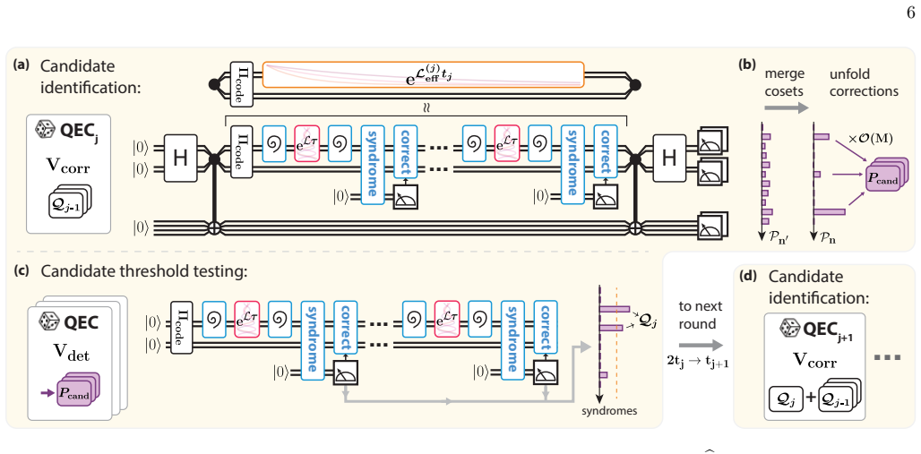
69 Algorithm 5:HDD Hamiltonian candidate identification subroutine,jth round Inputs : (1) Hierarchical round indexj
Leteρdenote the state immediately before Bell-basis measurement, eρ:= (etLeff ⊗I n′) (Π⊗I n′)ρ0(Π⊗I n′) tr((Π⊗I n′)ρ0) . 69 Algorithm 5:HDD Hamiltonian candidate identification subroutine,jth round Inputs : (1) Hierarchical round indexj. (2) Access ton-qubit evolutione tL (Eq. (E1)), where|SD|=M D,|S H |=M H, and thusM≤M 2 D +M H. (3) The η-heavy dissipat...
-
[2]
(Coverage and size) With probability at least1−δj, bYj ⊇ Y j \ bS(j−1) HDD,η,| bYj|=O M2 log(M/δj)
-
[3]
(Total evolution time) The total evolution time underetL is ttot =N codesNmeast=O 2jM2 log(M/δj)
-
[4]
(Time resolution) The procedure only applieseLt for times at least tres :=τ= t Nreshape ≥Ω 1 M32j
-
[5]
(Number of experiments) The number of Bell-sampling experiments is Nexp =N codesNmeas =O M3 log(M/δj) . The number of interleaved QEC rounds is larger by a factorO M24j , while the number of raw state-preparation attempts is larger by a factoreO(M)due to the probabilistic projection to the code space before reshaping
-
[6]
(Ancilla cost) The procedure uses at mostn+ 5⌈log2(2M)⌉ancillary qubits in addition to thenprobe qubits
-
[7]
(Classical overhead) The classical cost is dominated by repeated QEC and is eO (n+M)M 54j . Proof. Most of the proof concerns item(1), namely coverage of the candidate set. Items(2)–(4)follow directly from the schedule, and items(5)–(6)are verified at the end. We first prove coverage. The candidate-identification subroutine has atwo-level coupon-collector...
-
[8]
Operationally, this is implemented by measuring the stabilizers on the left register and postselecting on the trivial syndrome
The left half ofρ0 is projected into the code corner algebra: ρcode := (Πi ⊗I n′)ρ0(Πi ⊗I n′) tr((Πi ⊗I n′)ρ0) . Operationally, this is implemented by measuring the stabilizers on the left register and postselecting on the trivial syndrome. Using Eq. (E10), the success probability of this post-selection is tr((Πi ⊗I n′)ρ0) = 1 |S| ≥ 1 4M .(E14) For the id...
-
[9]
cosine" ˆo− s ←ˆo− s +v·logical measurement of(i T P a)onρ(t i)// for half ofN exp sample
Coefficient learning via robust frequency estimation In this section, we describe Hamiltonian-Disjoint-from-Dissipator coefficient learning at the Heisenberg limit. Given the candidate setbYj produced by Bell sampling, the goal is twofold: estimate the coefficients of the true round-j terms and remove the false positives. This produces the updated setbS(j...
-
[10]
(Accuracy) With probability≥1−δ coeff, |bha −h a| ≤ε
-
[11]
(Total evolution time) The total evolution time underetL is ttot =O 1 ε log 1 δcoeff + log log 1 ε ,
-
[12]
(Time resolution) It only ever applieseLt fort≥t res, where tres = min i ti Nreshape(ti) = Ω ε M2 , 75
-
[13]
(Number of experiments) The total number of state preparations / evolutions is N(tot) exp =L N exp =O log 1 ε log 1 δcoeff + log log 1 ε
-
[14]
(Ancilla cost) The procedure usesO(logM )ancillary qubits for code padding and check measurements (the same code reused from the structure-learning round in whichPa was sampled)
-
[15]
Matching the QEC reshaping plus logical twirl generator Eq.(C15) with the effective-generator form from Eq
(Classical overhead) The classical cost is: eO n2M2/ε2 Proof. Matching the QEC reshaping plus logical twirl generator Eq.(C15) with the effective-generator form from Eq. (E4), we can write Leff(ρ) =−i[(h a +b a)P a, ρ] +L resid(ρ),|b a| ≤B ∞,∥L resid∥⋄ ≤R ⋄. Let ωa := ha + ba. We first analyze RFE under the ideal unitary evolutione−iωaP at, and then accou...
-
[16]
Even though the algorithm closely follows [39], the complexity is different due to the underlying QEC-based Lindbladian reshaping
Full HDD hierarchical learning algorithm In this section, we combine candidate identification (Algorithm 5) and coefficient learning (Algorithm 6) into the full Hamiltonian-Disjoint-from-Dissipator learning Algorithm 7 according to Appendix E1. Even though the algorithm closely follows [39], the complexity is different due to the underlying QEC-based Lind...
-
[17]
(Accuracy) With probability at least1−δ, ∥bhHDD,η −h HDD,η∥∞ ≤ε
-
[18]
(Evolution time) The total evolution time underetL is ttot = eO M2 ε
-
[19]
(Time resolution) The procedure only appliesetL for times at least tres = Ω ε M3
-
[20]
(Number of experiments) The total number of collected measurements is eO M3 , dominated by Bell sampling during the candidate-identification stage. 79
-
[21]
(Ancilla cost) The procedure uses at most n+O(logM) noiseless ancilla qubits in addition to thenprobe qubits
-
[22]
The first and second terms come from real-time QEC processing in the candidate-identification stage, while the last term comes from logical-Pauli sampling in coefficient learning
(Classical overhead) The classical processing cost is eO M6 +nM 5 +n 2M4 ε2 . The first and second terms come from real-time QEC processing in the candidate-identification stage, while the last term comes from logical-Pauli sampling in coefficient learning. Proof.We first verify correctness. Since2−j ≥ε for all rounds j < L h, the uniform assumptionsB∞ ≤ε...
-
[23]
Hamiltonian disjoint from the dissipator
Removing the known dissipator structure assumption The conditional HDD Hamiltonian learner in Theorem E.3 takes theη-heavy dissipator structure as input and assumes that, after setting Vcorr = SD,η in the QEC reshaping routines, the resulting effective generators have sufficiently small bias and residual parametersB∞, K∞ and R⋄. We now remove this known-s...
-
[24]
Write it in the jump unraveling picture using Eq.(E7)and Eq.(E6): Leff(ρ) =−iH effρ+iρH † eff + X w,m αwmPwρPm, H eff :=H tar +H bias − i 2 Kresid
Deferred proofs for HDD Bell-sampling identification Restatement of Lemma E.6(Hamiltonian Bell sampling under bias and residual dissipation).Let Leff be an n′- qubit effective generator of the form in Eq.(E4), with bias and residual parametersB∞, K∞ as in Eq.(E7). Write it in the jump unraveling picture using Eq.(E7)and Eq.(E6): Leff(ρ) =−iH effρ+iρH † ef...
-
[25]
For any PauliP∈P n′, let OP := (P⊗I n′) |Φ0⟩ ⟨Φ0| (P † ⊗I n′)denote the corresponding Bell-measurement projector
Leteρdenote the state immediately before Bell-basis measurement, eρ:= (etLeff ⊗I n′) (Π⊗I n′)ρ0(Π⊗I n′) tr((Π⊗I n′)ρ0) . For any PauliP∈P n′, let OP := (P⊗I n′) |Φ0⟩ ⟨Φ0| (P † ⊗I n′)denote the corresponding Bell-measurement projector. Then, fort= 2 j/(2M), a single Bell-sampling experiment oneρsatisfies Pr(sampleP r modulo stabilizers):= tr X s∈S OsPreρ !...
-
[26]
Unless stated otherwise, operators act on the left register only, i.e.A≡A⊗IR
Operator content of the Lindbladian Choi state We work onHL ⊗ HR withnBell pairs, |Φ+⟩= 1√ 2(|00⟩+|11⟩), ρ 0 = |Φ+⟩ ⟨Φ+| ⊗n . Unless stated otherwise, operators act on the left register only, i.e.A≡A⊗IR. 88 Expanding the Lindbladian Choi stateEt(ρ0) := (etL ⊗I R)(ρ0)to first order in time gives Et(ρ0) =ρ 0 +tL(ρ 0) +O t2 =ρ 0 1− X Pm∈SD ammt ! − X Pk∈SH i...
-
[27]
The goal of the classical shadows is to estimate properties of a quantum stateρ using a small number of single-copy measurements
Review of classical shadows The key subroutine we use for learning the Lindbladian coefficients is the classical shadows protocol [90]. The goal of the classical shadows is to estimate properties of a quantum stateρ using a small number of single-copy measurements. The key step in the classical shadows algorithm involves creating a classical representatio...
-
[28]
Standard-Quantum-Limited coefficient learning We now formulate the coefficient-learning task for arbitrary specified Lindbladian coefficients. LetZH ⊆ P n \ {I} be the set of Hamiltonian Paulis whose coefficients we wish to estimate, and letZD ⊆ {(Pl, Pm) : Pl, Pm ∈ P n \{I}, l≥m} be the set of Kossakowski matrix entries whose coefficients we wish to esti...
-
[29]
(Accuracy) With probability≥1−δ, |bhk −h k| ≤ϵ,|ba lm −a lm| ≤ϵ for allP k ∈ Z H and all(P l, Pm)∈ Z D
-
[30]
(Evolution time) It applieseLt for total evolution time ttot =O ΛL ϵ2 log ΛL ϵ 7 log Nobs log(ΛL/ϵ) δ ! . 92
-
[31]
(Time resolution) It only ever applieseLtq fort q such that tq = Ω 1 ΛL log(ΛL/ϵ)2 ! andmin 1≤q≤r |tq+1 −t q|= Ω 1 ΛL log(ΛL/ϵ)2 !
-
[32]
(Number of experiments) It uses Nexp =O Λ2 L ϵ2 log ΛL ϵ 7 log Nobs log(ΛL/ϵ) δ ! quantum circuits, each preparingn Bell pairs, evolving one register undereLt for some t∈ (0, τmax), applying global random Clifford measurements on the resulting2n-qubit Choi state, and measuring in the computational basis
-
[33]
(Classical overhead) A direct implementation using a phase-sensitive Clifford simulator has classical post-processing cost eO Nexp(n3 +N obsn2) , whereN exp is the number of Choi-state classical-shadow snapshots in item(4). Proof. If Nobs = 0, the algorithm returns empty estimate lists and the claim is trivial, so assumeNobs ≥ 1. Throughout this proof, we...
discussion (0)
Sign in with ORCID, Apple, or X to comment. Anyone can read and Pith papers without signing in.