An Analysis of Posterior Collapse, Parameterization and Initialization in Variational Deep Gaussian Processes
Pith reviewed 2026-06-25 20:11 UTC · model grok-4.3
The pith
The linear prior mean in variational DGPs improves optimization conditioning at initialization rather than avoiding non-injective pathology.
A machine-rendered reading of the paper's core claim, the machinery that carries it, and where it could break.
Core claim
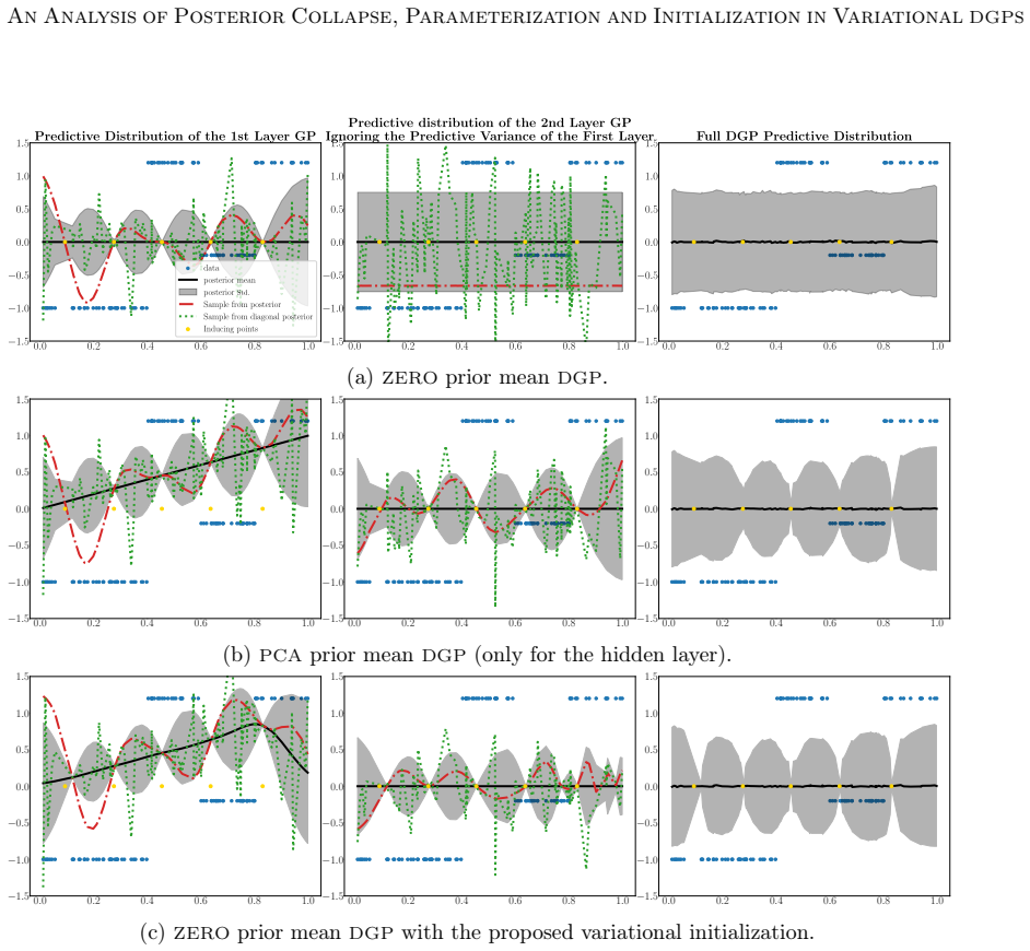
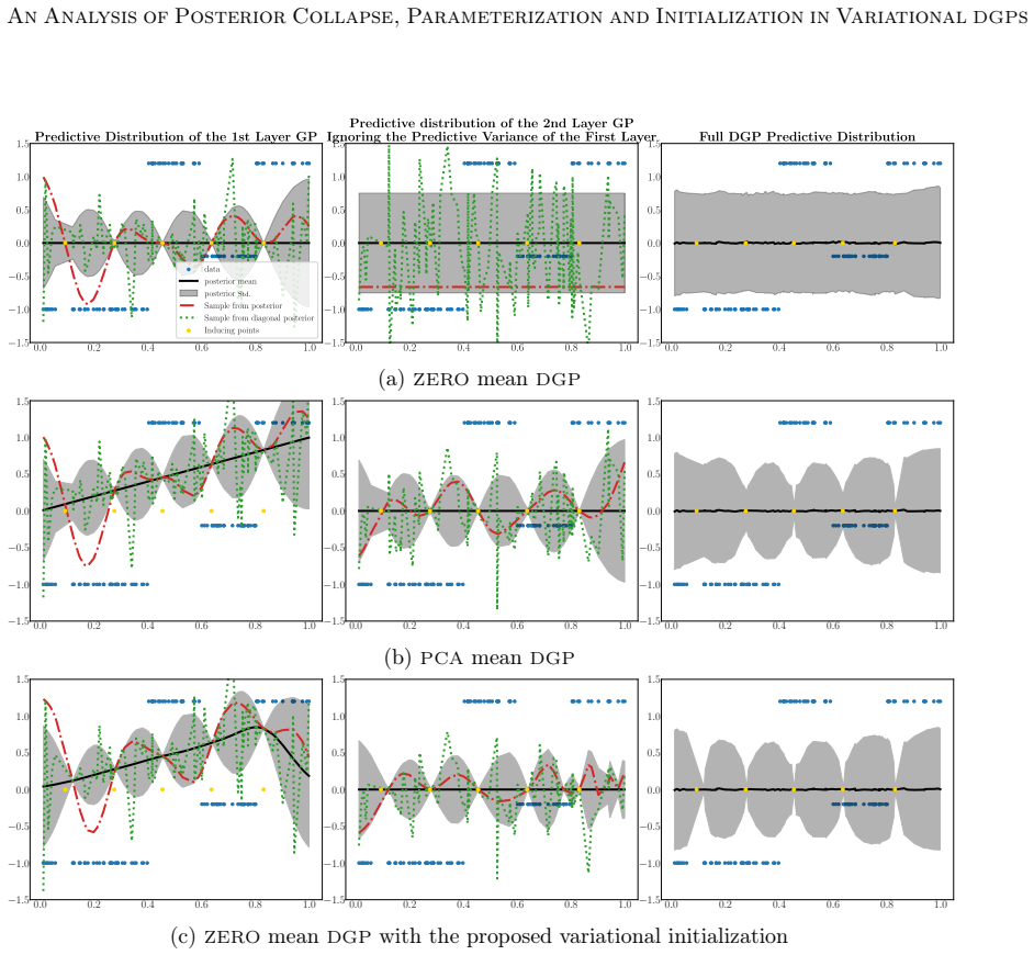
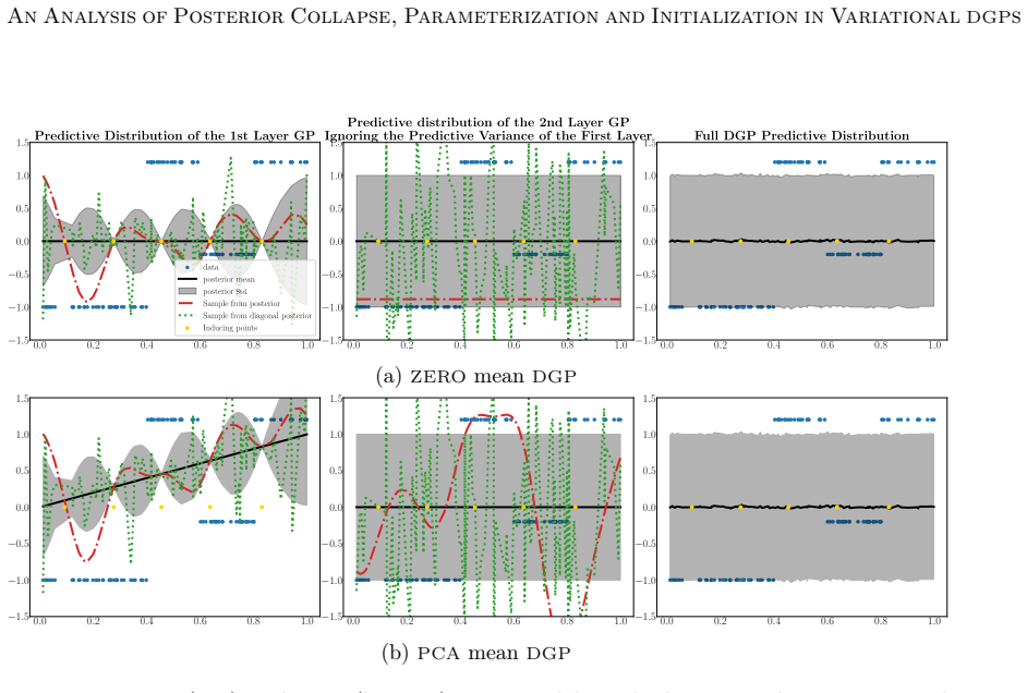
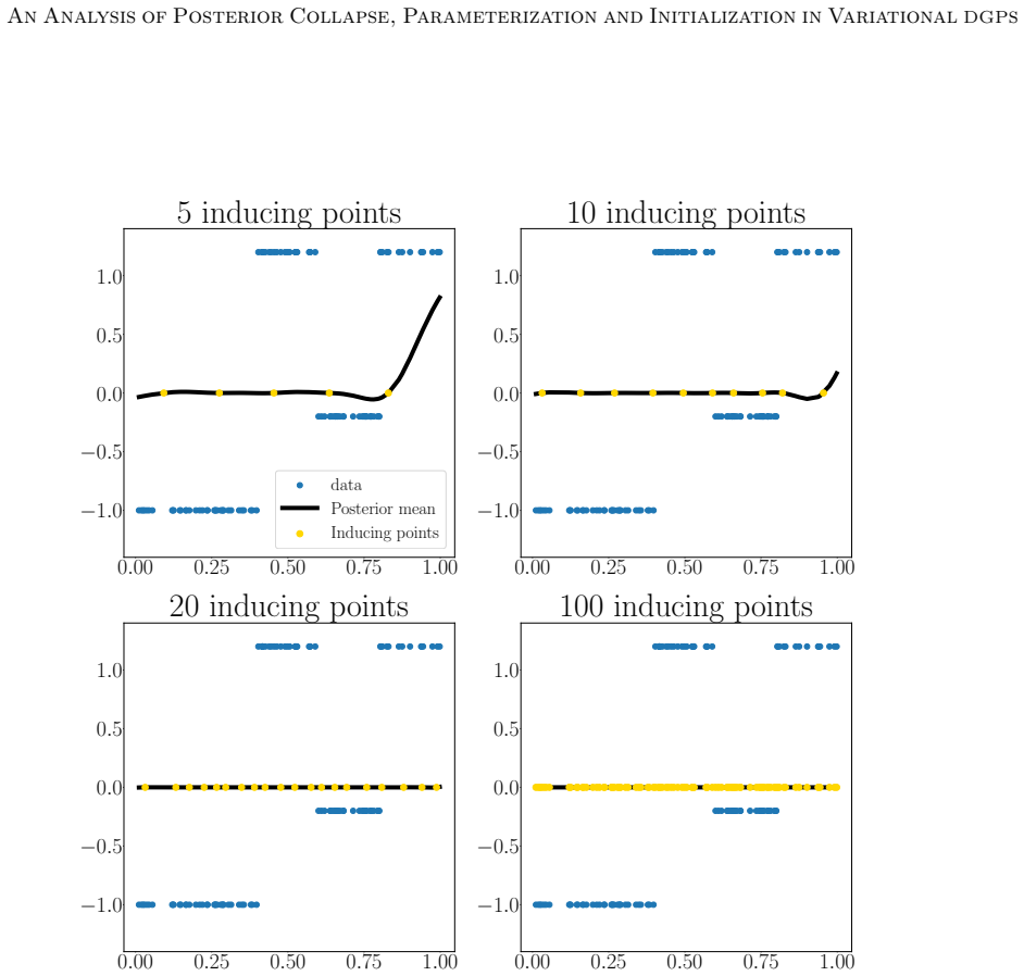
The benefit of the linear prior mean function does not arise from avoiding the non-injective pathology in very deep DGPs, as previously believed, but from improving the conditioning of the optimization problem at initialization. An alternative zero prior mean initialization that mimics a linear prior mean DGP at initialization enables successful training of DGPs without imposing optimization-driven constraints on the prior, and this initialization prevents posterior collapse while achieving performance comparable to or better than the linear-mean version across the studied parameterizations.
What carries the argument
The zero prior mean initialization strategy that matches linear-mean conditioning at the first training step, together with the analysis linking DSVI, linear prior means, and posterior collapse across three parameterizations.
If this is right
- DGPs can be trained without forcing the prior to satisfy optimization convenience.
- Whitened parameterizations yield more stable convergence and reduce posterior collapse risk.
- Not every DGP parameterization benefits equally from a linear prior mean.
- The proposed initialization yields performance comparable to or better than the linear-mean baseline.
Where Pith is reading between the lines
- Similar initialization-focused fixes may apply to posterior collapse in other variational deep models.
- The relative importance of the first training step could be tested by varying step size or optimizer in controlled ablations.
- Allowing priors to be set purely by modeling assumptions may change how practitioners choose mean functions in other Gaussian process models.
Load-bearing premise
The optimization dynamics at the first training step dominate the entire training trajectory for the three parameterizations.
What would settle it
A controlled experiment showing that zero-mean initialized DGPs still exhibit posterior collapse even when their initial conditioning matches that of linear-mean DGPs.
Figures


read the original abstract
DGPs are probabilistic models with remarkable prediction performance that concatenate GPs across several layers. Exact inference in DGPs is intractable, and variational inference is often used to approximate the posterior with a parametric distribution tuned by minimizing the Kullback-Leibler divergence. Moreover, finding a good VI approximation is challenging. In particular, a problem of VI is posterior collapse, where VI converges to a variational posterior that matches the prior. In variational DGPs, this implies explaining the data as noise. This work studies posterior collapse in DGPs and identifies its connection to the DSVI algorithm and the widely used linear prior mean function employed in all but the last layer. We show that the benefit of the linear prior mean does not arise from avoiding the non-injective pathology in very deep DGPs, as previously believed, but from improving the conditioning of the optimization problem at initialization. Thus, we propose an alternative initialization of a zero prior mean DGP that mimics a DGP with a linear prior mean at initialization. This enables successful training of DGPs without imposing optimization-driven constraints on the prior, allowing to choose the prior based on modeling assumptions rather than optimization convenience. Our analysis considers three common parameterizations of DGPs and shows that not all of them benefit from a linear prior mean. We also explain why a whitened parameterization of the \DGP provides more stable convergence, something often assumed from experience, but lacking a rigorous analysis. Furthermore, we show that this stability is also beneficial to avoid the posterior collapse problem. Extensive experiments validate our findings: the proposed initialization prevents posterior collapse, improves stability, and achieves performance comparable to (and sometimes better than) DGPs with a linear prior mean.
Editorial analysis
A structured set of objections, weighed in public.
Referee Report
Summary. The paper analyzes posterior collapse in variational deep Gaussian processes (DGPs) under three common parameterizations. It argues that the benefit of the linear prior mean function (used in all but the final layer) arises from improving the conditioning of the optimization problem at initialization rather than from avoiding non-injective pathologies in deep models. The authors propose an alternative zero-mean initialization that mimics the linear-mean DGP at step zero, claim this prevents collapse while allowing modeling-driven prior choice, provide an analysis of why the whitened parameterization yields more stable convergence, and report that experiments confirm comparable or better performance without the linear-mean constraint.
Significance. If the initialization equivalence holds across the full optimization trajectory, the work would allow DGPs to be trained with priors chosen for modeling reasons rather than optimization convenience, while supplying a rigorous account of whitened-DGP stability that is currently assumed from experience. The explicit comparison across standard, whitened, and other parameterizations is a clear strength; the derivation linking DSVI, linear means, and conditioning at initialization is also potentially useful if the trajectory-level claim is substantiated.
major comments (2)
- [Abstract and initialization analysis sections] The central substitution of a zero-mean initialization for the linear prior mean rests on the unverified assumption that first-step conditioning benefits dominate the entire training trajectory for all three parameterizations. No derivation or experiment is shown establishing that the variational parameters or inducing-point posteriors remain aligned after the first gradient update; if later steps allow the zero-mean model to escape the well-conditioned basin, the performance equivalence fails.
- [Experiments section] The claim that the proposed initialization prevents posterior collapse and achieves comparable performance is supported only by the statement that 'extensive experiments validate our findings.' Without reported details on data splits, quantitative metrics, baselines, or controls for post-hoc choices, it is impossible to assess whether the results actually establish trajectory-level equivalence rather than initial-value equivalence.
minor comments (1)
- [Abstract] The abstract contains the notation '\DGP'; this should be rendered consistently as 'DGP' throughout.
Simulated Author's Rebuttal
We thank the referee for their detailed and constructive comments on our manuscript. We address each of the major comments below and have made revisions to strengthen the paper accordingly.
read point-by-point responses
-
Referee: [Abstract and initialization analysis sections] The central substitution of a zero-mean initialization for the linear prior mean rests on the unverified assumption that first-step conditioning benefits dominate the entire training trajectory for all three parameterizations. No derivation or experiment is shown establishing that the variational parameters or inducing-point posteriors remain aligned after the first gradient update; if later steps allow the zero-mean model to escape the well-conditioned basin, the performance equivalence fails.
Authors: We acknowledge that our primary analysis focuses on the benefits at initialization. While the manuscript presents empirical evidence from extensive experiments showing that the proposed initialization prevents posterior collapse and achieves comparable performance, we agree that a more rigorous examination of the parameter trajectories would provide stronger support for the claim that the benefits persist throughout training. In the revised manuscript, we will include additional experiments that track the evolution of variational parameters and inducing point posteriors over the course of optimization for both initializations. revision: yes
-
Referee: [Experiments section] The claim that the proposed initialization prevents posterior collapse and achieves comparable performance is supported only by the statement that 'extensive experiments validate our findings.' Without reported details on data splits, quantitative metrics, baselines, or controls for post-hoc choices, it is impossible to assess whether the results actually establish trajectory-level equivalence rather than initial-value equivalence.
Authors: The experiments section of the manuscript does provide details on the datasets, metrics, and comparisons, but we recognize that the presentation may not have been sufficiently explicit or comprehensive. To address this, we will revise the experiments section to include more detailed descriptions of the experimental setup, including data splits, quantitative results with standard deviations, baseline comparisons, and controls to demonstrate that the performance equivalence holds beyond the initial step. revision: yes
Circularity Check
No circularity; analysis grounded in standard DSVI/DGP formulations and external experiments
full rationale
The paper examines posterior collapse via connections to the existing DSVI algorithm and linear prior mean functions used in prior DGP literature. The proposed zero-mean initialization is motivated by mimicking behavior at step 0 and is validated empirically across three parameterizations, without defining any quantities in terms of fitted outputs or renaming predictions. No load-bearing self-citations, uniqueness theorems imported from the authors' prior work, or ansatzes smuggled via citation appear in the derivation. The central claims rest on analysis of standard formulations and experimental benchmarks rather than reducing to self-defined inputs by construction, making the work self-contained against external validation.
Axiom & Free-Parameter Ledger
axioms (2)
- domain assumption Variational inference via minimization of KL divergence between variational posterior and true posterior yields a valid approximation for DGPs.
- domain assumption The DSVI algorithm is a correct instantiation of variational inference for the DGP model class.
Reference graph
Works this paper leans on
-
[1]
URLhttps://arxiv.org/abs/2410.08315. M. Bauer, M. van der Wilk, and C. E. Rasmussen. Understanding Probabilistic Sparse Gaussian Process Approximations. InAdvances in Neural Information Processing Systems, pages 1533 – 1541,
-
[2]
URLhttps://arxiv.org/abs/2104.05674. D. Duvenaud, O. Rippel, R. Adams, and Z. Ghahramani. Avoiding pathologies in very deep networks. InInternational Conference on Artificial Intelligence and Statistics, pages 202–210,
-
[3]
M. Havasi, J. M. Hernández-Lobato, and J. J. Murillo-Fuentes. Inference in Deep Gaussian Processes using Stochastic Gradient Hamiltonian Monte Carlo. InAdvances in Neural Information Processing Systems, pages 7517 – 7527, 2018a. M. Havasi, J. M. Hernández-Lobato, and J. J. Murillo-Fuentes. Deep Gaussian Processes with Decoupled Inducing Inputs, 2018b. URL...
-
[4]
URLhttps://arxiv.org/abs/1905.13697. A. Javaloy, M. Meghdadi, and I. Valera. Mitigating Modality Collapse in Multimodal VAEs via Impartial Optimization. InInternational Conference on Machine Learning, pages 9938–9964,
Pith/arXiv arXiv 1905
-
[5]
URLhttps://arxiv.org/abs/2012.13962. Z. Lin, F. Yin, and J. Maroñas. Towards Flexibility and Interpretability of Gaussian Process State-Space Model,
arXiv 2012
-
[6]
URLhttps://arxiv.org/abs/2301.08843. J. Z. Liu, S. Padhy, J. Ren, Z. Lin, Y. Wen, G. Jerfel, Z. Nado, J. Snoek, D. Tran, and B. Lakshminarayanan. A Simple Approach to Improve Single-Model Deep Uncertainty via Distance-Awareness.Journal of Machine Learning Research, 24:1–63,
-
[7]
URLhttps://arxiv.org/abs/ 2506.23996. A. G. d. G. Matthews, M. van der Wilk, T. Nickson, K. Fujii, A. Boukouvalas, P. León- Villagrá, Z. Ghahramani, and J. Hensman. GPflow: A Gaussian Process library using TensorFlow.Journal of Machine Learning Research, 18:1–6, apr
-
[8]
URLhttps://arxiv.org/abs/2010.14877. C. E. Rasmussen and C. K. I. Williams.Gaussian Processes for Machine Learning. The MIT Press,
arXiv 2010
-
[9]
F. J. Sáez-Maldonado, J. Maroñas, and D. Hernández-Lobato. Mode Collapse in Variational Deep Gaussian Processes. InNeurIPS 2024 Workshop on Bayesian Decision-making and Uncertainty,
2024
-
[10]
J. Shi, M. Titsias, and A. Mnih. Sparse Orthogonal Variational Inference for Gaussian Processes. InInternational Conference on Artificial Intelligence and Statistics, pages 1932–1942,
1932
-
[11]
URLhttps://arxiv.org/abs/2310.18230. M. Titsias. Variational Learning of Inducing Variables in Sparse Gaussian Processes. In International Conference on Artificial Intelligence and Statistics, pages 567–574,
-
[12]
URLhttps: //arxiv.org/abs/2003.01115. Y. Wang, D. Blei, and J. P. Cunningham. Posterior Collapse and Latent Variable Non- identifiability. InAdvances in Neural Information Processing Systems, pages 5443–5455,
arXiv 2003
-
[13]
80 An Analysis of Posterior Collapse, Parameterization and Initialization in V ariationalDGPs Appendix A
ISSN 1935-8237. 80 An Analysis of Posterior Collapse, Parameterization and Initialization in V ariationalDGPs Appendix A. Coordinate Updates for the Noise Parameter By noting that a one-dimensional Gaussian likelihood function can be compactly expressed through: NY n=1 N yn |f n, σ2 =N Y|f, σ 2I (75) The objective function of a one-dimensionalSVGPcan be w...
1935
-
[14]
Model KLDLik. Var.RMSE ZERO-W 0.0010 0.9967 0.9896 ZERO-NWR 869.0811 1.1559 0.9895 PCA-W 144.5761 0.00530.0420 PCA-NWR 3310.1553 1.1707 0.9895 ZERO-Points-M0-W 184.2085 0.0058 0.0580 ZERO-Points-M0-NWR 92017.6629 1.0156 0.9903 ZERO-Points-MY-W 144253.7899 0.0321 0.0946 ZERO-Points-MY-NWR 2164.8801 1.5375 0.9901 Table 9: Test metrics achieved by all the me...
arXiv 2085
discussion (0)
Sign in with ORCID, Apple, or X to comment. Anyone can read and Pith papers without signing in.