Unbiased Hamiltonian Simulation by Reversing Trotter Error Dynamics
Pith reviewed 2026-06-30 06:29 UTC · model grok-4.3
The pith
Trotter error reversal via quasi-probabilistic sampling produces unbiased Hamiltonian simulation.
A machine-rendered reading of the paper's core claim, the machinery that carries it, and where it could break.
Core claim
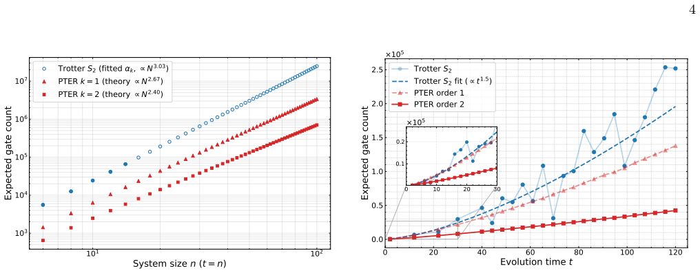
The Trotter error is itself a coherent dynamics to be reversed, rather than a deviation to be bounded. By identifying the structure of this error in a suitable form, reversal is carried out through quasi-probabilistic decompositions. The resulting Probabilistic Trotter Error Reversal (PTER) algorithm is unbiased, improves the gate-count scaling compared to Suzuki-Trotter formulas, and retains their simplicity.
What carries the argument
Probabilistic Trotter Error Reversal (PTER) that reverses the coherent Trotter error dynamics using quasi-probabilistic decompositions.
If this is right
- The simulation produces unbiased results matching the exact unitary evolution in expectation.
- Gate count scales better than standard Suzuki-Trotter methods for the same accuracy.
- The method applies to any order k of Trotter formula.
- Numerical simulations of Heisenberg spin chains show resource advantage at modest sizes.
Where Pith is reading between the lines
- This method could be combined with other error mitigation techniques in quantum computing.
- Applications may extend to simulating more complex Hamiltonians where Trotter errors are prominent.
- Further optimization of the quasi-probabilistic decomposition might reduce the sampling overhead.
Load-bearing premise
The Trotter error can be expressed in a form that permits reversal by quasi-probabilistic sampling.
What would settle it
Running the PTER algorithm on a small quantum system and observing that the measured expectation values deviate systematically from the exact result beyond statistical error.
Figures

read the original abstract
Owing to their simplicity and low overhead, Suzuki--Trotter formulas remain the de facto Hamiltonian simulation methods on current quantum computing platforms. Systematic Trotter errors, however, will quickly become limiting when scaling to larger problems and aiming for higher accuracy. We present a mechanism that removes the systematic error of any $k$-th order Suzuki--Trotter simulation, at the cost of a constant sampling overhead. The key insight is that the Trotter error is itself a coherent dynamics to be reversed, rather than a deviation to be bounded. By identifying the structure of this error in a suitable form, we carry out that reversal through quasi-probabilistic decompositions. The resulting algorithm, called Probabilistic Trotter Error Reversal (PTER), is unbiased, improves the gate-count scaling compared to Suzuki--Trotter formulas, and still retains their simplicity. Numerical simulations of a Heisenberg spin chain support the predicted resource advantage already at modest system sizes.Keisuke Murota, Yuta Kikuchi, Enrico Rinaldi, Fr\'ed\'eric Sauvage, Synge Todo
Editorial analysis
A structured set of objections, weighed in public.
Referee Report
Summary. The paper introduces Probabilistic Trotter Error Reversal (PTER), which removes the systematic bias of any k-th order Suzuki-Trotter product formula by treating the Trotter error as a coherent dynamics that can be exactly reversed via a quasi-probabilistic decomposition into implementable unitaries. The resulting estimator is unbiased, incurs only constant sampling overhead independent of simulation time t and system size, and improves the asymptotic gate-count scaling relative to standard Trotter formulas while preserving their structural simplicity. Numerical experiments on a Heisenberg spin chain are presented as supporting evidence for the predicted resource advantage at modest sizes.
Significance. If the constant-overhead claim holds, the method would allow Trotter-based simulations to achieve higher accuracy without the usual error-accumulation penalty, potentially extending the practical reach of near-term quantum devices for Hamiltonian simulation. The paper explicitly credits the retention of algorithmic simplicity and provides numerical support at small system sizes; these are concrete strengths. However, the significance is tempered by the need to confirm that the quasi-probabilistic l1-norm remains bounded independently of t and N.
major comments (2)
- [Abstract / key insight paragraph] Abstract and the paragraph beginning 'The key insight is that the Trotter error is itself a coherent dynamics': the assertion that the sampling overhead remains constant independent of t, system size, and Trotter order k is load-bearing for both the unbiasedness and improved-scaling claims. The error term itself scales as O(t^{k+1}), so any exact reversal must either absorb this growth into the coefficients or exploit a cancellation whose l1-norm bound is shown to be O(1). No explicit bound or scaling argument is referenced in the provided abstract; this requires a concrete derivation or theorem statement.
- [Numerical simulations (Heisenberg chain)] Numerical simulations section (Heisenberg chain): the abstract states that the simulations 'support the predicted advantage,' yet the reader's report notes the absence of error bars, dataset sizes, or exclusion criteria. Because the central unbiasedness claim rests on the quasi-probabilistic reversal working exactly, the numerical evidence must demonstrate that the observed variance matches the predicted constant overhead rather than growing with t; without these controls the support is inconclusive.
minor comments (2)
- [Abstract] The abstract refers to 'improves the gate-count scaling' without specifying the new scaling exponent relative to the original k-th order Trotter formula; a brief comparison (e.g., effective order or prefactor) would clarify the improvement.
- Notation for the quasi-probabilistic coefficients and the associated sampling procedure should be introduced with a short equation or definition early in the manuscript to aid readability.
Simulated Author's Rebuttal
We thank the referee for the constructive comments on our manuscript. We address each major comment below, indicating the revisions that will be incorporated.
read point-by-point responses
-
Referee: [Abstract / key insight paragraph] Abstract and the paragraph beginning 'The key insight is that the Trotter error is itself a coherent dynamics': the assertion that the sampling overhead remains constant independent of t, system size, and Trotter order k is load-bearing for both the unbiasedness and improved-scaling claims. The error term itself scales as O(t^{k+1}), so any exact reversal must either absorb this growth into the coefficients or exploit a cancellation whose l1-norm bound is shown to be O(1). No explicit bound or scaling argument is referenced in the provided abstract; this requires a concrete derivation or theorem statement.
Authors: We agree that the abstract should reference the supporting result. The full manuscript contains Theorem 1, which derives that the l1-norm of the quasi-probability distribution implementing the error reversal is bounded by a constant depending only on k (specifically, at most 2^{O(k)} but independent of t and N). The proof proceeds by expressing the leading Trotter error as a linear combination of unitaries whose coefficients permit an exact quasi-probabilistic decomposition without t-dependent growth in the norm. We will revise the abstract to cite this theorem and state the constant-overhead bound explicitly. revision: yes
-
Referee: [Numerical simulations (Heisenberg chain)] Numerical simulations section (Heisenberg chain): the abstract states that the simulations 'support the predicted advantage,' yet the reader's report notes the absence of error bars, dataset sizes, or exclusion criteria. Because the central unbiasedness claim rests on the quasi-probabilistic reversal working exactly, the numerical evidence must demonstrate that the observed variance matches the predicted constant overhead rather than growing with t; without these controls the support is inconclusive.
Authors: We accept that additional statistical details are needed for clarity. In the revised manuscript we will add error bars (computed from 10^4 independent circuit executions per data point), state the sample sizes explicitly, and confirm that no data were excluded. These controls will show that the empirical variance remains flat with t, consistent with the constant-overhead prediction, thereby strengthening the numerical support. revision: yes
Circularity Check
No significant circularity detected
full rationale
The paper presents PTER as a new quasi-probabilistic reversal of Trotter error dynamics, building on but independent of standard Suzuki-Trotter formulas. No equations, fitted parameters, or self-citations are shown that reduce the claimed unbiased simulation or constant-overhead improvement to a self-referential definition or input fit. The derivation chain remains self-contained, with the central mechanism (identifying error structure for reversal) not reducing by construction to prior results or data subsets within the provided text.
Axiom & Free-Parameter Ledger
axioms (1)
- standard math Suzuki-Trotter formulas provide a valid approximation to time evolution under a Hamiltonian
Reference graph
Works this paper leans on
-
[1]
throughMrepeated measurements. Errors in such estimates are quantified by the root-mean-square error, RMSE = q bias2 + ∆2 1s/M ,(16) that captures the systematic error (bias) and the statis- tical fluctuation (variance) given by the single-shot vari- ance ∆2 1s rescaled by the number of measurements [30]. The following studies compare the expected gate co...
-
[2]
R. P. Feynman, Simulating physics with computers, International Journal of Theoretical Physics21, 467 (1982)
1982
-
[3]
Lloyd, Universal quantum simulators, Science273, 1073 (1996)
S. Lloyd, Universal quantum simulators, Science273, 1073 (1996)
1996
-
[4]
Savary and L
L. Savary and L. Balents, Quantum spin liquids: A re- view, Rep. Prog. Phys.80, 016502 (2017)
2017
-
[5]
M. C. Ba˜ nuls, R. Blatt, J. Catani, A. Celi, J. I. Cirac, M. Dalmonte, L. Fallani, K. Jansen, M. Lewenstein, S. Montangero, C. A. Muschik, B. Reznik, E. Rico, L. Tagliacozzo, K. Van Acoleyen, F. Verstraete, U.-J. Wiese, M. Wingate, J. Zakrzewski, and P. Zoller, Sim- ulating lattice gauge theories within quantum technolo- gies, European Physical Journal D...
2020
-
[6]
McArdle, S
S. McArdle, S. Endo, A. Aspuru-Guzik, S. C. Benjamin, and X. Yuan, Quantum computational chemistry, Rev. Mod. Phys.92, 015003 (2020)
2020
-
[7]
M. L. Baez, M. Goihl, J. Haferkamp, J. Bermejo-Vega, M. Gluza, and J. Eisert, Dynamical structure factors of dynamical quantum simulators, Proc. Natl. Acad. Sci. U.S.A.117, 26123 (2020)
2020
-
[8]
E. H. Lieb and D. W. Robinson, The finite group velocity of quantum spin systems, Communications in Mathemat- ical Physics28, 251 (1972)
1972
- [9]
- [10]
-
[11]
H. F. Trotter, On the product of semi-groups of opera- tors, Proceedings of the American Mathematical Society 10, 545 (1959)
1959
-
[12]
M. Suzuki, Generalized Trotter’s formula and systematic approximants of exponential operators and inner deriva- tions with applications to many-body problems, Commu- nications in Mathematical Physics51, 183 (1976)
1976
-
[13]
Suzuki, General theory of fractal path integrals with applications to many-body theories and statistical physics, Journal of Mathematical Physics32, 400 (1991)
M. Suzuki, General theory of fractal path integrals with applications to many-body theories and statistical physics, Journal of Mathematical Physics32, 400 (1991)
1991
-
[14]
A. M. Childs, Y. Su, M. C. Tran, N. Wiebe, and S. Zhu, Theory of Trotter error with commutator scaling, Phys. Rev. X11, 011020 (2021)
2021
-
[15]
A. M. Childs, D. Maslov, Y. Nam, N. J. Ross, and Y. Su, Toward the first quantum simulation with quan- tum speedup, Proc. Natl. Acad. Sci. U.S.A.115, 9456 (2018)
2018
-
[16]
G. H. Low and I. L. Chuang, Optimal Hamiltonian Sim- 6 ulation by Quantum Signal Processing, Phys. Rev. Lett. 118, 010501 (2017)
2017
-
[17]
A. Gily´ en, Y. Su, G. H. Low, and N. Wiebe, Quan- tum singular value transformation and beyond: expo- nential improvements for quantum matrix arithmetics, inProceedings of the 51st Annual ACM SIGACT Sympo- sium on Theory of Computing(ACM, 2019) pp. 193–204, arXiv:1806.01838
-
[18]
G. H. Low and I. L. Chuang, Hamiltonian Simulation by Qubitization, Quantum3, 163 (2019)
2019
-
[19]
D. W. Berry, G. Ahokas, R. Cleve, and B. C. Sanders, Ef- ficient quantum algorithms for simulating sparse Hamil- tonians, Communications in Mathematical Physics270, 359 (2007), arXiv:quant-ph/0508139
work page internal anchor Pith review Pith/arXiv arXiv 2007
-
[20]
D. W. Berry, A. M. Childs, and R. Kothari, Hamiltonian simulation with nearly optimal dependence on all param- eters, inProceedings of the 56th Annual IEEE Symposium on Foundations of Computer Science (FOCS)(2015) pp. 792–809, arXiv:1501.01715 [quant-ph]
work page internal anchor Pith review Pith/arXiv arXiv 2015
-
[21]
Campbell, Random Compiler for Fast Hamiltonian Simulation, Phys
E. Campbell, Random Compiler for Fast Hamiltonian Simulation, Phys. Rev. Lett.123, 070503 (2019)
2019
-
[22]
A. M. Childs, A. Ostrander, and Y. Su, Faster quantum simulation by randomization, Quantum3, 182 (2019)
2019
-
[23]
Chen, H.-Y
C.-F. Chen, H.-Y. Huang, R. Kueng, and J. A. Tropp, Concentration for random product formulas, PRX Quan- tum2, 040305 (2021)
2021
- [24]
-
[25]
M. Pocrnic, M. Hagan, J. Carrasquilla, D. Segal, and N. Wiebe, Composite Qdrift-product formulas for quan- tum and classical simulations in real and imaginary time, Phys. Rev. Res.6, 013224 (2024), arXiv:2306.16572 [quant-ph]
- [26]
- [27]
-
[28]
Granet and H
E. Granet and H. Dreyer, Hamiltonian dynamics on digi- tal quantum computers without discretization error, npj Quantum Information10, 82 (2024)
2024
-
[29]
Chakraborty, Implementing any linear combination of unitaries on intermediate-term quantum computers, Quantum8, 1496 (2024)
S. Chakraborty, Implementing any linear combination of unitaries on intermediate-term quantum computers, Quantum8, 1496 (2024)
2024
-
[30]
Kiumi and B
C. Kiumi and B. Koczor, Te-pai: exact time evolution by sampling random circuits, Quantum Science and Tech- nology10, 045071 (2025)
2025
- [31]
-
[32]
Continuous-time evolution via probabilistic angle interpolation and its applications
T. Hayata and Y. Kikuchi, Continuous-time evolution via probabilistic angle interpolation and its applications (2026), arXiv:2604.02854 [quant-ph]
work page internal anchor Pith review Pith/arXiv arXiv 2026
-
[33]
P. Zeng, J. Sun, L. Jiang, and Q. Zhao, Simple and high- precision hamiltonian simulation by compensating trot- ter error with linear combination of unitary operations, PRX Quantum6, 010359 (2025)
2025
-
[34]
Koczor, J
B. Koczor, J. J. Morton, and S. C. Benjamin, Probabilis- tic interpolation of quantum rotation angles, Phys. Rev. Lett.132, 130602 (2024)
2024
-
[35]
It relates to the form quoted in the main text simply by taking the adjoint of the circuits
In fact, we detail the circuit implementation of Q1(τ) †[·]Q1(τ). It relates to the form quoted in the main text simply by taking the adjoint of the circuits
-
[36]
The gate counts of the individual sampled circuits concentrate around this expected value with a standard deviation p E[Ng] according to the Poisson dis- tribution
All the gate counts quoted in this work are expected countsE[N g]. The gate counts of the individual sampled circuits concentrate around this expected value with a standard deviation p E[Ng] according to the Poisson dis- tribution
-
[37]
Fauseweh, Quantum many-body simulations on digi- tal quantum computers: State-of-the-art and future chal- lenges, Nature Communications15, 2123 (2024)
B. Fauseweh, Quantum many-body simulations on digi- tal quantum computers: State-of-the-art and future chal- lenges, Nature Communications15, 2123 (2024)
2024
-
[38]
Miessen, P
A. Miessen, P. J. Ollitrault, F. Tacchino, and I. Taver- nelli, Quantum algorithms for quantum dynamics, Na- ture Computational Science3, 25 (2023)
2023
-
[39]
M. Heyl, P. Hauke, and P. Zoller, Quantum localization bounds Trotter errors in digital quantum simulation, Sci- ence Advances5, eaau8342 (2019)
2019
-
[40]
Layden, First-order Trotter error from a second- order perspective, Phys
D. Layden, First-order Trotter error from a second- order perspective, Phys. Rev. Lett.128, 210501 (2022), arXiv:2107.08032 [quant-ph]
-
[41]
M. Hagan and N. Wiebe, Composite quantum simula- tions, Quantum7, 1181 (2023), arXiv:2206.06409 [quant- ph]
- [42]
-
[43]
N. Yoshioka, T. Okubo, Y. Suzuki, Y. Koizumi, and W. Mizukami, Hunting for quantum-classical crossover in condensed matter problems, npj Quantum Informa- tion10, 45 (2024), arXiv:2210.14109 [quant-ph]
-
[44]
A. Carrera Vazquez, D. J. Egger, D. Ochsner, and S. Woerner, Well-conditioned multi-product formulas for hardware-friendly Hamiltonian simulation, Quantum7, 1067 (2023), arXiv:2207.11268
- [45]
-
[46]
Lin and Y
L. Lin and Y. Tong, Heisenberg-limited ground-state en- ergy estimation for early fault-tolerant quantum comput- ers, PRX Quantum3, 010318 (2022)
2022
-
[47]
A. Dutkiewicz, S. Polla, M. Scheurer, C. Gogolin, W. J. Huggins, and T. E. O’Brien, Error mitigation and circuit division for early fault-tolerant quantum phase estima- tion, PRX Quantum6, 040318 (2025), arXiv:2410.05369 [quant-ph]
- [48]
- [49]
-
[50]
D. Aharonov, X. Gao, Z. Landau, Y. Liu, and U. Vazi- rani, A Polynomial-Time Classical Algorithm for Noisy Random Circuit Sampling, in55th Annual ACM Sympo- sium on Theory of Computing(2022) arXiv:2211.03999 [quant-ph]
-
[51]
E. Fontana, M. S. Rudolph, R. Duncan, I. Rungger, and C. Cˆ ırstoiu, Classical simulations of noisy varia- tional quantum circuits, npj Quantum Inf.11, 84 (2025), arXiv:2306.05400 [quant-ph]
-
[52]
Watrous,The Theory of Quantum Information(Cam- bridge University Press, Cambridge, 2018)
J. Watrous,The Theory of Quantum Information(Cam- bridge University Press, Cambridge, 2018)
2018
-
[53]
Quantum Circuits with Mixed States
D. Aharonov, A. Kitaev, and N. Nisan, Quantum cir- cuits with mixed states, inProceedings of the 30th An- nual ACM Symposium on Theory of Computing (STOC) 7 (1998) pp. 20–30, arXiv:quant-ph/9806029
work page internal anchor Pith review Pith/arXiv arXiv 1998
-
[54]
J. Haah, R. Kothari, R. O’Donnell, and E. Tang, Query- optimal estimation of unitary channels in diamond dis- tance, in2023 IEEE 64th Annual Symposium on Founda- tions of Computer Science (FOCS)(2023) pp. 363–390, arXiv:2302.14066 [quant-ph]. 8 Appendix The appendix is organised in five parts. Sec. A derives a nested-commutator representation of the remai...
-
[55]
Suzuki–Trotter formulas We recall the Suzuki–Trotter product formulas [12, 13] that are used later on. For a Hamiltonian decomposed as H= LX ℓ=1 Hℓ,(A1) with eachH ℓ being a weighted sum of mutually commuting Pauli strings, the first- and second-order formulas read S1(τ) := LY ℓ=1 e−iτ Hℓ , S2(τ) := LY ℓ=1 e−i τ 2 Hℓ 1Y ℓ=L e−i τ 2 Hℓ . (A2) Higher even o...
-
[56]
Definition of the remainder HamiltonianG k In this section we derive a first expression for the remainder HamiltonianGk at arbitrarykand discuss its properties. Splitting the total evolution timetintorsteps of lengthτ=t/r, we define within a single step thecorrection unitary as a function of the running times∈[0, τ], Qk(s) :=U(s)S † k(s),(A10) so thatU(s)...
-
[57]
(A15) at first (k= 1), second (k= 2), and general orderkall rely on a single operator-calculus identity: the integral-remainder expansion of e −itad X (Y), which we now detail
Tool: the conjugation identity The following derivations ofG k in Eq. (A15) at first (k= 1), second (k= 2), and general orderkall rely on a single operator-calculus identity: the integral-remainder expansion of e −itad X (Y), which we now detail. For an arbitrary operatorX, the commutator map ad X is defined by adX(Y) := [X, Y] =XY−Y X,(A17) and the conju...
-
[58]
First order:G 1 At first order,S 1(s) = e−iAse−iBs. The Trotter generator is given by HS(s) = i(∂sS1)S † 1 = e−isad A(A+B).(A23) 11 Likewise, the conjugated Hamiltonian decomposes as S1(s)HS † 1(s) = e−isad A e−isad B(A) +B .(A24) Substituting the two previous equalities into Eq. (A15), one gets G1(s) =−e −isad A e−isad B(A)−A .(A25) Applying Eq. (A20) wi...
-
[59]
Second order:G 2 We now deriveG 2(s) for the second-order Trotter formulaS 2(s) = e−iA s 2 e−iBs e−iA s 2 . DifferentiatingS 2(s) gives HS(s) = i(∂sS2)S † 2 = 1 2 A+ e −i s 2 adA(B) + 1 2e−i s 2 adA e−isad B(A) .(A28) In addition, the conjugated Hamiltonian forH=A+Bdecomposes as S2(s)HS † 2(s) = e−i s 2 adAe−isad B A+ e −i s 2 adA(B) .(A29) In turn, Eq. (...
-
[60]
First, we rewriteG k(s) as a sum of conjugated Hamiltonian terms
Generalk: commutator kernel form This subsection proves Lemma 2 of the main text, and proceeds in three parts. First, we rewriteG k(s) as a sum of conjugated Hamiltonian terms. Second, we recall the commutator-expansion theorem of Childs et al. [13], which expands a conjugation by a product of matrix exponentials as a polynomial insof degreek−1 together w...
-
[61]
For now, let us drop the time dependence for ease of notation
Unbiased channel simulation and Hermitian-involution decompositions Consider a time-dependent HamiltonianH(s) and the corresponding Hamiltonian evolution (as a unitary) for a timet, U(t) =Texp −i Z t 0 H(s) ds .(B1) Further define the evolution channelU(t)[·] =U(t)(·)U(t) †. For now, let us drop the time dependence for ease of notation. We say that a set{...
-
[62]
decomposition of the form Eq
TE-PAI TE-PAI is one instantiation of QPDs for Hamiltonian evolution under a time-dependent Hamiltonian with h.i. decomposition of the form Eq. (B6). Following Ref. [33], the time evolutionU(t)[ρ] is first approximated by a first- order Trotter formula (for time-dependent Hamiltonians) U(t)[ρ]≈ NτY µ=1 Y j e−iθjµ Rj ρ NτY µ=1 Y j e−iθjµ Rj † ,(B7) with ro...
-
[63]
Implementation We first draw an integerN g from a Poisson distribution with the expected number of events given by Eq. (B15). The integerN g indicates the number of non-identity channels (i.e. the number of rotations, or gate count) in a circuit. For each insertionm∈ {1,2, . . . , N g}:
-
[64]
Draw a timet m ∈[0, τ] from the densityp(t) = P j |cj(t)|/λ(B15)
-
[65]
Draw a labeljof a Hamiltonian term with probability (conditioned ont m)p(j) =|c j(tm)|/P j′ |cj′(tm)|
-
[66]
Apply the sampled channels in increasing order of sampled timest m to obtain one circuit instance, of overall sign ε= QNg m=1 εm
PickR j(sgn(cj(tm))∆) with probabilityp 2/(p2+p3) (B11) andR j(π) otherwise, and retain the signε m = sgn(γl) of the corresponding coefficient in (B9). Apply the sampled channels in increasing order of sampled timest m to obtain one circuit instance, of overall sign ε= QNg m=1 εm. Following the quasi-probabilistic estimator (B4), the value of the observab...
-
[67]
replaceV→V /r
Resources: per-step gate count andr-step composition We now collect the resources used by TE-PAI to implement a single step of unitary evolution of lengthτ, then describe how they compose whenrsuch primitives are employed in a given circuit. Already, the expected number of non-identity channels (i.e., the gate count) per circuit was provided in Eq. (B15)....
-
[68]
(B18), which is the integrated 1-norm of the Hamiltonian in the chosen h.i
Pauli-basis integrated rate The resource required by TE-PAI (Lemma 5) is controlled by the integrated rate of Eq. (B18), which is the integrated 1-norm of the Hamiltonian in the chosen h.i. decomposition. To implement the correction channel, we use the standard Pauli basis to decompose the remainder HamiltonianG k(s), so that the integrated rateλ k is def...
-
[69]
Let us first evaluate the gate count for PTERk at a fixed number of stepsr=t/τ
Gate-count optimisation This subsection proves Theorems 1 and 2 of the main text and relies on the scaling of the integrated rateλ k(τ) obtained in the previous subsection. Let us first evaluate the gate count for PTERk at a fixed number of stepsr=t/τ. ImplementingU(t) =U(τ) r requiresrsteps of Trotter circuits, interleaved withrsteps of TE-PAI correction...
-
[70]
LetH= PL ℓ=1 Hℓ, where eachH ℓ is a weighted sum of mutually commuting Pauli strings, otherwise arbitrary
Gate count for non-local Hamiltonians We now drop the geometric-locality assumption of the previous subsection. LetH= PL ℓ=1 Hℓ, where eachH ℓ is a weighted sum of mutually commuting Pauli strings, otherwise arbitrary. The proof of Lemma 6 used geometric locality to show that, when conjugating any of the Pauli strings appearing in the commutatorsC ν by th...
-
[71]
B 3 were based on knowledge of a Hermitian-involution (h.i.) decomposition of the remainder Hamiltonian (B6) such as Gk(s) = X j cj(s)R j,(D1) with{R j}a set of h.i
Preamble The implementation items of TE-PAI presented in Sec. B 3 were based on knowledge of a Hermitian-involution (h.i.) decomposition of the remainder Hamiltonian (B6) such as Gk(s) = X j cj(s)R j,(D1) with{R j}a set of h.i. operators (for instance, Pauli strings). Given such a decomposition, one obtains the 1-norm of the Hamiltonian at any times, ∥Gk(...
-
[72]
Geometrically local case: explicit Pauli decomposition For the geometrically local case, recasting the generator (D4) into an explicit Pauli decomposition is relatively straightforward. In Sec. D 2 a, we detail how we obtain the explicit Pauli decomposition ofG 1(s) that can be used for the implementation of TE-PAI (and thus PTER) for the simplified setti...
-
[73]
(D8) and thus in Eq
Non-local case: Pauli-path sampler For non-local Hamiltonians the previous approach could fail: we are not guaranteed any more that only a constant number of rotations act non-trivially, such that we may have an exponentially large number of contributing Pauli strings appearing in Eq. (D8) and thus in Eq. (D1). To overcome this problem we will resort to a...
-
[74]
Draw a times m ∈[0, τ] from the densityp(s) =∥G 1(s)∥1,spath/¯λ1, with∥G 1(s)∥1,spath defined in Eq. (D25)
-
[75]
From this, obtain the Pauli stringP xm together with the weightsg(x m) (D12) and ¯g(xm) (D19)
Draw an extended pathx m = (hm, Sm, σm) from the alternative tree distribution (D22). From this, obtain the Pauli stringP xm together with the weightsg(x m) (D12) and ¯g(xm) (D19)
-
[76]
Pick the sign of the PauliP xm to bea m =±1 with probability p(am|xm) = ¯gxm(s) +a mgxm(s) 2 ¯gxm(s) .(D27)
-
[77]
PickR xm(am∆) with probabilityp 2/(p2 + p3) (B11) andR xm(π) otherwise, and retain the signε m = sgn(γl) of the corresponding coefficient in (B9)
Define the Pauli-rotation channelR xm(θ)[·] := e −iθPxm [·]eiθPxm . PickR xm(am∆) with probabilityp 2/(p2 + p3) (B11) andR xm(π) otherwise, and retain the signε m = sgn(γl) of the corresponding coefficient in (B9). Apply theN g sampled channels in increasing order of sampled timess m to obtain one circuit instance, of overall sign ε= QNg m=1 εm (the path ...
discussion (0)
Sign in with ORCID, Apple, or X to comment. Anyone can read and Pith papers without signing in.