REVIEW 1 major objections 4 minor 78 references
Construction of Green's functions on a quantum computer: applications to molecular systems
T0 review · 1 major / 4 minor · reviewed 2026-08-14 · deepseek-v4-flash
Pith's one-line read This paper claims that a quantum computer can construct the one-particle Green's function of an interacting molecular system through statistical sampling: specially built circuits probabilistically prepare electron-added and…
desk verdict Solid, honest algorithm paper for molecular Green's functions on a quantum computer; the eigenstate caveat is real but disclosed. read the letter →
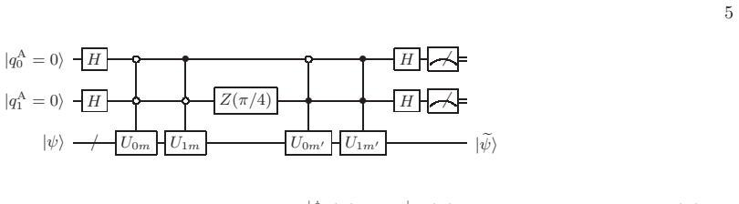
The pith
A machine-rendered reading of the paper's core claim, the machinery that carries it, and where it could break.
The reading
What carries the argument
The load-bearing object is the probabilistic state-preparation circuit, built on the Majorana-like decomposition of the fermionic creation and annihilation operators into two unitaries: $a_m^\dagger = (U_{0m} - U_{1m})/2$ and $a_m = (U_{0m} + U_{1m})/2$, with $U_{0m}$ and $U_{1m}$ the combinations of Pauli operations from the Jordan–Wigner or Bravyi–Kitaev representation. Circuit $C_m$ uses one ancilla and controlled $U_{0m}$, $U_{1m}$ to entangle the ancilla with the register; post-selecting on the ancilla outcome yields the normalized electron-added or electron-removed state. Circuit $C_{mm'}$ uses two ancillas and the phase-shifted auxiliary operators $a^{\pm}_{mm'} = (a_m \pm e^{-i\pi/4} a_{m'})/2$ to reach the off-diagonal amplitudes. These circuits convert the non-unitary action of $a_m^\dagger$ and $a_m$ into a unitary operation on a larger Hilbert space, which is exactly what a quantum circuit can implement. The subsequent QPE histogram then reads out the transition matrix elements as probabilities.
What would settle it
Construct the Green's function for LiH on a device with a deliberately coarse quantum phase estimation register and compare the pole positions of the reconstructed spectrum with the exact FCI spectrum: any shift beyond the known statistical sampling error would falsify the assumption of perfect QPE precision.
Extended reading notes
Core claim
On the paper's own terms, the central discovery is that the Lehmann representation of the one-particle Green's function can be evaluated by sampling rather than by computing overlaps. Because $a_m^\dagger \pm a_m$ are unitary by the fermionic anticommutation relations, one writes $a_m^\dagger = (U_{0m} - U_{1m})/2$ and $a_m = (U_{0m} + U_{1m})/2$, and a controlled circuit $C_m$ entangles an ancilla with the register so that measuring the ancilla leaves $|0\rangle \otimes a_m|\psi\rangle$ or $|1\rangle \otimes a_m^\dagger|\psi\rangle$. Feeding the result into quantum phase estimation turns the histogram of measured (ancilla, energy) pairs into the diagonal transition elements $B^{(e)}_{\lambda mm}$ and $B^{(h)}_{\lambda mm}$ (eqs. 25–26); the two-ancilla circuit $C_{mm'}$ similarly yields the off-diagonal elements through auxiliary operators $a^{\pm}_{mm'}$. The full Green's function then follows by inserting these $B$'s and the known $(N \pm 1)$-electron energies into the Lehmann sums (eqs. 3–4).
Load-bearing premise
The scheme assumes the energy eigenvalues of the $(N \pm 1)$-electron states are already known exactly and that quantum phase estimation returns them with no error; in addition, the input state is treated as an exact eigenstate of the Hamiltonian, which the UCC trial states used here are not.
Editorial extensions
If this is right
- The same sampling scheme can be applied to any ground state that a quantum computer can prepare, not just UCC states, since the circuits only need the state as input.
- The full Green's function, including quasiparticle and satellite peaks, can be reconstructed on a quantum computer using at most two ancilla qubits, regardless of system size.
- Total energies can be extracted from the sampled Green's function via the Galitskii–Migdal formula, converging to the expected value as the number of measurements grows.
- The scheme converts the problem of computing transition matrix elements into one of counting histogram bins, a purely classical post-processing task.
Reading between the lines
- A natural extension is to replace the ideal QPE with finite-resolution phase estimation; the resulting pole shifts would turn the ideal-precision assumption into a concrete resource estimate for the required energy-register accuracy.
- The same probabilistic-preparation trick might be adapted to other non-unitary operations in quantum simulation, such as projecting onto symmetry sectors or implementing imaginary-time evolution steps.
- For strongly correlated molecules, where satellite weights are large, the number of measurements needed to resolve them may scale unfavorably; the paper's LiH and H2O data already hint at this, and a formal scaling bound would be a testable follow-up.
Signed reviews
Editorial analysis
A structured set of objections, weighed in public.
Referee Report
Summary. The paper proposes a scheme for constructing the one-particle Green's function (GF) of a molecular system on a quantum computer via statistical sampling. The key idea is to encode creation and annihilation operators as linear combinations of unitaries, so that circuits C_m and C_{mm'} probabilistically prepare electron-added and electron-removed states. After the ancilla measurement, quantum phase estimation (QPE) projects onto (N±1)-electron energy eigenstates, and the histogram frequencies directly give the diagonal and off-diagonal transition matrix elements B^{(e/h)}_{λmm'} that enter the Lehmann representation. The authors demonstrate the sampling procedure in classical simulations for LiH and H2O using unitary coupled-cluster (UCC) trial states, comparing the sampled spectra with spectra 'exact within UCC' and with FCI spectra, and they analyze convergence of Galitskii-Migdal correlation energies as the number of measurements grows.
Significance. If the claims are taken as stated, the paper provides a simple and explicit circuit-level method for the previously missing ingredient in quantum-computing approaches to spectral functions: the measurement of the numerators of the Lehmann representation. The algebraic derivations in Eqs. (8)-(20) are internally consistent, and the probability counting in Eqs. (25)-(28) correctly recovers the transition matrix elements. The classical sampling simulations are honest Monte Carlo experiments with no fitted parameters, and the pseudocodes make the protocol reproducible. The main weakness, discussed below, is that the object computed for a UCC reference state is not the exact Green's function of the prepared state, which limits the physical interpretation of the demonstrated spectra.
major comments (1)
- [II.B.1 and IV.A.2] The Lehmann representation in Eqs. (3) and (4) is derived under the assumption that |Ψ_N_gs⟩ is an eigenstate of H with energy E_N_gs. The UCC trial states used in Secs. IV.A.1 and IV.B.1 are not eigenstates of H. For a non-eigenstate |Ψ_UCC⟩, the resolvent expression ⟨Ψ_UCC| a_m (z+E_ref-H)^{-1} a†_{m'} |Ψ_UCC⟩ contains an additional sum over all N-electron eigenstates, and no choice of E_ref makes Eqs. (3)-(4) exact. The assembled object is therefore not the one-particle Green's function of the system, but rather a model GF defined by the trial state and the trial energy. The paper acknowledges the associated discrepancy for the Galitskii-Migdal formula in Sec. II.C, but the abstract and Sec. IV present the sampled spectra as the GF of an interacting electronic system and compare them with FCI spectra without a clear statement of this approximation. The authors should revise the claims to distinguish the exact case (exact ground state prepared) from the approximate demonstration (UCC state), and ideally quantify the error of the trial-state GF relative to the exact resolvent GF of |Ψ_UCC⟩.
minor comments (4)
- [III] The paper uses classical FCI eigenvalues for the (N±1)-electron states and assumes ideal QPE. Since the algorithm's output is the transition matrix elements, not the poles, the authors should state more prominently that the complete GF construction requires a separate accurate determination of the (N±1) spectra; the current text says this in Sec. III, but the abstract's phrasing could mislead readers.
- [II.B.4] The pseudocode in Procedures 2-4 instructs 'Find E among {E^{N±1}_λ}' after QPE. Under ideal precision this is fine, but with finite-precision QPE the eigenvalue estimate will not exactly coincide with a known eigenvalue; a brief discussion of binning and the associated pole-shift error would make the protocol more complete.
- [II.B.3] In Eq. (20), the appearance of the phase gate Z(π/4) and the factor e^{iπ/4} in the resulting state is not derived; spelling out the connection between the phase gate and the definitions in Eqs. (13)-(14) would improve readability.
- [Throughout] There are minor typographical issues, e.g., 'ancillae' is used where 'ancillas' is standard, and 'H2O' is used without subscript in some places; these do not affect the technical content.
Circularity Check
Sampled spectra are Monte Carlo re-draws of the exact transition matrix elements; the circuit derivation itself is independent.
-
self definitional
[Section IV A 3 (LiH); same sampling procedure for H2O in Sec. IV B 3; target AUCC defined in Sec. IV A 2.]
"We generated random numbers according to these values since they represent the probability distributions of the measurement results for the qubits. [See eqs. (25)-(28)] By building the histograms of the results of simulated measurements, we constructed the GF GUCC−stat for the UCC ground state."
The 'these values' are the exact transition matrix elements B(e/h)λmm, which are also the amplitudes used in eqs. (3)-(4) to define the exact-within-UCC spectrum AUCC. The simulated measurement outcomes are therefore random draws from the very distribution that defines the target spectrum, so GUCC−stat converges to AUCC by the law of large numbers. Consequently the agreement shown in Figs. 5(b) and 7(b), and the GM-energy convergence in Figs. 6(b) and 8(b), demonstrates Monte Carlo consistency of the sampling procedure rather than an independent validation of the circuit/QPE construction. The analytic circuit identities (25)-(28) remain non-circular; the by-construction loop is confined to the numerical demonstration of validity.
full rationale
The central derivation is self-contained: the probabilities of the QPE outcomes after circuits Cm and Cmm' are shown analytically to equal the transition matrix elements B(e/h) (eqs. 25-28), and the denominator poles are supplied as known FCI energies, an explicitly stated assumption rather than a fitted output. UCC parameters are optimized to the N-electron ground-state energy, not to spectral weights, so they do not bias the sampled B values. The only reduction-by-construction is the validation loop described above: the simulation draws random numbers from the exact B values and then compares the resulting histograms with spectra built from those same B values. This is a low-severity self-consistency check, not a failure of the proposed algorithm. The non-eigenstate UCC issue is acknowledged in Sec. II C ('EGM[Gtrial] ... can differ from the expected energy ... since eqs. (3) and (4) use the fact that the true ground state is an eigenstate of H'); it is an approximation/limitation and a correctness risk, not a circular step. No load-bearing self-citation or imported uniqueness theorem appears. Score 4 reflects the one statistically forced numerical prediction while the central circuit identities retain independent content.
Assumptions & free parameters
free parameters (3)
- LiH UCC ansatz parameters θ1, θ2 =
not listed; result EUCC1 = -214.3323 eV
- H2O UCC ansatz parameters θ1..θ6 =
not listed; result EUCC1 = -2040.4359 eV
- Spectral broadening δ =
0.02 a.u.
assumptions (4)
- standard math For JW and BK transformations, every creation and annihilation operator can be written as (U0-U1)/2 and (U0+U1)/2 with unitary U0, U1.
- domain assumption The N-electron input state |Ψgs⟩ can be prepared on the quantum computer (e.g., via VQE/UCC).
- domain assumption The energy eigenvalues of the (N±1)-electron states are known exactly, and QPE operates with ideal precision.
- ad hoc to paper Each cluster operator in the UCC ansatz is approximated by a single Pauli tensor per parameter.
Cite this review
Pith. "Pith review of Construction of Green's functions on a quantum computer: applications to molecular systems." pith.science (2026). https://pith.science/paper/HFUBG7VS
@misc{pith2026190803902,
  author       = {Pith},
  title        = {Pith review of: Construction of Green's functions on a quantum computer: applications to molecular systems},
  year         = {2026},
  howpublished = {\url{https://pith.science/paper/HFUBG7VS}},
  note         = {Machine review of arXiv:1908.03902}
}
abstract
We propose a scheme for the construction of one-particle Green's function (GF) of an interacting electronic system via statistical sampling on a quantum computer. Although the non-unitarity of creation and annihilation operators for the electronic spin orbitals prevents us from preparing specific states selectively, probabilistic state preparation is demonstrated to be possible for the qubits. We provide quantum circuits equipped with at most two ancillary qubits for obtaining all the components of GF. We perform simulations of such construction of GFs for LiH and H$_2$O molecules based on the unitary coupled-cluster (UCC) method to demonstrate the validity of our scheme by comparing the spectra exact within UCC and those from full configuration interaction calculations. We also examine the accuracy of sampling method by exploiting the Galitskii--Migdal formula, which gives the total energy only from the GF.
Figures


Figures from the paper (5 more)


Reference graph
Works this paper leans on
-
[1]
Definition Although we assume the ground state |Ψ N gs⟩ to be non- degenerate and to be at zero temperature for simplicity, the expressions provided below are easily extended for systems having degenerate ground states at nonzero tem- perature. The one-particle GF[ 41, 42] of the system in frequency domain is given by Gmm′ (z) = G(e) mm′(z) +G(h) mm′(z) (2...
-
[2]
In the 3 present case, one might think by looking at eq
Circuits for diagonal components In a typical scheme for the construction of GFs on a classical computer[ 25–29], the equation-of-motion coupled-cluster (EOM-CC) approach is adopted to ob- tain the energy eigenvalues and the transition matrix ele- ments for the (N ±1)-electron intermediate states. In the 3 present case, one might think by looking at eq. (...
-
[3]
and ( 4), provided that the denominators have been known
-
[4]
The whole system consists of the ancilla and an arbitrary input register |ψ ⟩, whose state changes by undergoing the circuit as |0⟩ ⊗ |ψ ⟩ ↦− → |0⟩ ⊗U0m +U1m 2 |ψ ⟩ + |1⟩ ⊗U0m −U1m 2 |ψ ⟩ = |0⟩ ⊗am|ψ ⟩ + |1⟩ ⊗a† m|ψ ⟩ ≡ |Φ m⟩. (10) The action of the circuit to the whole system is easily confirmed to be unitary due to the anti-commutation re- lation between...
-
[5]
Circuits for off-diagonal components For the mth and m′th spin orbitals ( m ⁄= m′), we define the following auxiliary creation and annihilation operators a± mm′ ≡ am ±e−iπ/ 4am′ 2 (13) and a±† mm′ ≡ a† m ±eiπ/ 4a† m′ 2 , (14) respectively, which are the Hermitian conjugate of each other. Unnormalized auxiliary ( N + 1)-electron states |Ψ (e)± mm′⟩ ≡a±† mm′|...
-
[6]
S. B. Bravyi and A. Y. Kitaev, Annals of Physics 298, 210 (2002)
2002
-
[7]
Transition matrices via statistical sampling Given the results of measurement on the ancillary bit(s), we have the register |~ψ ⟩ representing the Ne- electron state with Ne = N + 1 or N − 1. Then we perform QPE by inputting |~ψ ⟩ to obtain the energy eigen- value in the subspace spanned by the Ne-electron states. A QPE experiment inevitably suffers from p...
-
[8]
D. S. Abrams and S. Lloyd, Phys. Rev. Lett. 79, 2586 (1997)
1997
Show all 78 references
-
[9]
D. S. Abrams and S. Lloyd, Phys. Rev. Lett. 83, 5162 (1999)
1999
-
[10]
( 3) and ( 4) use the fact that the true ground state is an eigenstate of H
and ( 4) can differ from the expected energy in general: EGM[Gtrial] ⁄= ⟨Ψ trial|H|Ψ trial⟩ , since eqs. ( 3) and ( 4) use the fact that the true ground state is an eigenstate of H. We use the expressions in eqs. ( 31) and ( 32), however, to exam- ine quantitatively the accurac...
-
[11]
We set δ in eq
and ( 4). We set δ in eq. ( 7) to 0. 02 a.u. for the spec- tral functions throughout the present study. For numerical evaluation of the integrals in eqs. ( 30) and ( 32), we adopted rectangular contours on the com- plex plane so that they encircle all the poles on the neg- ati...
-
[12]
6 ˚ A in an LiH molecule, we performed an RHF calculation and ob- tained ERHF = −213
UCC calculations By fixing the bond length at 1 . 6 ˚ A in an LiH molecule, we performed an RHF calculation and ob- tained ERHF = −213. 9322 eV and six spatial orbitals among which the two lowest ones were fully occupied. Therefore we adopted the RHF solution as the reference s...
-
[13]
The opti- mizedU1 gaveEUCC1 = −214
It is similarly the case with CLiH 2 . The opti- mizedU1 gaveEUCC1 = −214. 3323 eV, closer to the FCI value EFCI = −214. 4889 eV than the optimized U2 did with EUCC2 = −213. 9758 eV
-
[14]
GFs exact within UCC We calculated the GFs from the ground states of the FCI and optimized UCC solutions, as shown in Fig. 5 (a). The FCI spectra AFCI(ω ) exhibit the weak satellite peaks, which are correlation effects and thus are absent 7 H2O molecule (a) (b) LiH molecule Orb...
-
[15]
The satellite peaks are also seen in the UCC spectra AUCC(ω ) for both U1 and U2. The quasiparticle peaks in the FCI spectra are closer to the Fermi level ( ω = 0) than the HF orbital energies are, which is due to the well known fact that HF solutions overestimate energy gaps ...
-
[16]
This means that we can calculate the off-diagonal component of B(h) λ fromD(h)± λ by using the same expression as eq
with (e) replaced by (h). This means that we can calculate the off-diagonal component of B(h) λ fromD(h)± λ by using the same expression as eq. ( 18) with the replacement. We construct a circuit Cmm′ equipped with two ancil- lary qubits |qA 0 ⟩ and |qA 1 ⟩ by implementing the c...
-
[17]
UCC GFs via statistical sampling Hereafter we denote the ground state for the opti- mized U1 simply by the UCC ground state |Ψ N (UCC) gs ⟩. To simulate the scheme for obtaining GFs on a quantum computer proposed above, we calculated the transition matrix elements between |Ψ N...
-
[18]
It is easily con- firmed that ∑ σ =+, −[∑ λ ∈N −1pmm′(σ,E N −1 λ ) +∑ λ ∈N +1pmm′(σ,E N +1 λ )] = 1, as expected
via statistical sampling for a fixed combination of m and m′. It is easily con- firmed that ∑ σ =+, −[∑ λ ∈N −1pmm′(σ,E N −1 λ ) +∑ λ ∈N +1pmm′(σ,E N +1 λ )] = 1, as expected. We provide the pseudocodes in Appendix A for the calculation process of GF explained above. C. Galitski...
-
[19]
Correlation energy from GF To examine the statistical behavior of GUCC−stat quantitatively, we performed 100 simulations to obtain GUCC−stat for each given value of Nmeas and calcu- lated the correlation energies by using the GM for- mula in eqs. (
-
[20]
96 ˚ A and the H-O-H bond angle at 104
UCC calculations By fixing the O-H bond length at 0 . 96 ˚ A and the H-O-H bond angle at 104 . 5◦ in an H 2O molecule, we performed an RHF calculation and obtained ERHF = −2039. 8504 eV and seven spatial orbitals among which the five lowest ones were fully occupied. Therefore we...
2013
-
[21]
(28) This means that we can get the off-diagonal com- ponents of transition matrices B(e) λ and B(h) λ from eq
and ( 23)] pmm′(±,E N −1 λ ) = ⏐ ⏐ ⏐ ⏐ ⏐⟨Ψ N −1 λ | a± m′m √ pmm′(h, ±) |Ψ N gs⟩ ⏐ ⏐ ⏐ ⏐ ⏐ 2 pmm′(h, ±) = D(h)± λmm ′. (28) This means that we can get the off-diagonal com- ponents of transition matrices B(e) λ and B(h) λ from eq. (
-
[22]
GFs exact within UCC We calculated the GFs from the ground states of the FCI and optimized UCC solutions, as shown in Fig. 7 (a). These three spectral functions admit analyses similar to those for an LiH molecule described above, since an H 2O molecule is also a weakly correla...
-
[23]
We performed sim- ulations for obtaining GFs via statistical sampling in the same manner as in the case of an LiH molecule
UCC GFs via statistical sampling Hereafter we denote the ground state for the optimized U1 simply by the UCC ground state. We performed sim- ulations for obtaining GFs via statistical sampling in the same manner as in the case of an LiH molecule. Typical simulated spectral fun...
-
[24]
Correlation energy from GF Similarly to the case of an LiH molecule, we performed 100 simulations to obtain GUCC−stat for each given value ofNmeas and calculated the correlation energies by using the GM formula, as shown in Fig. 8(b). Although the increase in Nmeas leads to th...
-
[25]
McArdle, S
S. McArdle, S. Endo, A. Aspuru-Guzik, S. Benjamin, and X. Yuan, arXiv e-prints , arXiv:1808.10402 (2018), arXiv:1808.10402 [quant-ph]
2018 arXiv
-
[26]
Feynman, Int J Theor Phys 21, 467 (1982)
R. Feynman, Int J Theor Phys 21, 467 (1982)
1982
-
[27]
M. A. Nielsen and I. L. Chuang, Quantum Computation and Quantum Information: 10th Anniversary Edition , 10th ed. (Cambridge University Press, New York, NY, USA, 2011)
2011
-
[28]
J. T. Seeley, M. J. Richard, and P. J. Love, The Journal of Chemical Physics 137, 224109 (2012) , https://doi.org/10.1063/1.4768229
2012 doi
-
[29]
Jordan and E
P. Jordan and E. Wigner, Zeitschrift f¨ ur Physik47, 631 (1928)
1928
-
[30]
Aspuru-Guzik, A
A. Aspuru-Guzik, A. D. Dutoi, P. J. Love, and M. Head-Gordon, Science 309, 1704 (2005) , https://science.sciencemag.org/content/309/5741/1704.full.pdf
2005
-
[31]
The results for Nmeas = 1000, 2000, 4000, 8000, 16000, and 32000 are shown in Fig
and ( 32). The results for Nmeas = 1000, 2000, 4000, 8000, 16000, and 32000 are shown in Fig. 6(b), where ∆ E1[GUCC−stat] and ∆ E2[GUCC−stat] scatter around the ideal values, ∆ E1[GUCC] and ∆ E2[GUCC], respectively. The deviations of the sampled values from the ideal values de...
2000
-
[32]
Suzuki, Physics Letters A 165, 387 (1992)
M. Suzuki, Physics Letters A 165, 387 (1992)
1992
-
[33]
J. D. Whitfield, J. Biamonte, and A. Aspuru- Guzik, Molecular Physics 109, 735 (2011) , https://doi.org/10.1080/00268976.2011.552441
2011
-
[34]
P. J. J. O’Malley, R. Babbush, I. D. Kivlichan, J. Romero, J. R. McClean, R. Barends, J. Kelly, P. Roushan, A. Tranter, N. Ding, B. Campbell, Y. Chen, Z. Chen, B. Chiaro, A. Dunsworth, A. G. Fowler, E. Jef- frey, E. Lucero, A. Megrant, J. Y. Mutus, M. Nee- ley, C. Neill, C. Qu...
2016
-
[35]
J. R. McClean, J. Romero, R. Babbush, and A. Aspuru- Guzik, New Journal of Physics 18, 023023 (2016)
2016
-
[36]
Peruzzo, J
A. Peruzzo, J. McClean, P. Shadbolt, M.-H. Yung, X.-Q. Zhou, P. J. Love, A. Aspuru-Guzik, and J. L. O’Brien, Nature Communications 5, 4213 EP (2014) , article
2014
-
[37]
Kandala, A
A. Kandala, A. Mezzacapo, K. Temme, M. Takita, M. Brink, J. M. Chow, and J. M. Gambetta, Nature 549, 242 EP (2017)
2017
-
[38]
Hempel, C
C. Hempel, C. Maier, J. Romero, J. McClean, T. Monz, H. Shen, P. Jurcevic, B. P. Lanyon, P. Love, R. Bab- bush, A. Aspuru-Guzik, R. Blatt, and C. F. Roos, Phys. Rev. X 8, 031022 (2018)
2018
-
[39]
Jones, S
T. Jones, S. Endo, S. McArdle, X. Yuan, and S. C. Benjamin, Phys. Rev. A 99, 062304 (2019)
2019
-
[40]
McArdle, T
S. McArdle, T. Jones, S. Endo, Y. Li, S. C. Benjamin, and X. Yuan, npj Quantum Information 5, 75 (2019)
2019
-
[41]
X. Yuan, S. Endo, Q. Zhao, Y. Li, and S. C. Benjamin, Quantum 3, 191 (2019)
2019
-
[42]
McLachlan, Molecular Physics 8, 39 (1964) , https://doi.org/10.1080/00268976400100041
A. McLachlan, Molecular Physics 8, 39 (1964) , https://doi.org/10.1080/00268976400100041
1964 doi
-
[43]
Damascelli, Physica Scripta 2004, 61 (2004)
A. Damascelli, Physica Scripta 2004, 61 (2004)
2004
-
[44]
Moser, Journal of Electron Spectroscopy and Related Phenomena 214, 29 (2017)
S. Moser, Journal of Electron Spectroscopy and Related Phenomena 214, 29 (2017)
2017
-
[45]
Kosugi, H
T. Kosugi, H. Nishi, Y. Kato, and Y.-i. Matsushita, Journal of the Physical Society of Japan 86, 124717 (2017) , https://doi.org/10.7566/JPSJ.86.124717
2017 doi
-
[46]
Kosugi and Y.-I
T. Kosugi and Y.-I. Matsushita, Journal of Physics: Condensed Matter 30, 435604 (2018)
2018
-
[47]
Nooijen and J
M. Nooijen and J. G. Snijders, International Journal of Quantum Chemistry 44, 55 (1992) . 15
1992
-
[48]
Nooijen and J
M. Nooijen and J. G. Snijders, International Journal of Quantum Chemistry 48, 15 (1993)
1993
-
[49]
Nooijen and J
M. Nooijen and J. G. Snijders, The Journal of Chemical Physics 102, 1681 (1995) , https://doi.org/10.1063/1.468900
1995 doi
-
[50]
Kowalski, K
K. Kowalski, K. Bhaskaran-Nair, and W. A. Shelton, The Journal of Chemical Physics 141, 094102 (2014) , http://dx.doi.org/10.1063/1.4893527
2014 doi
-
[51]
Bhaskaran-Nair, K
K. Bhaskaran-Nair, K. Kowalski, and W. A. Shelton, The Journal of Chemical Physics 144, 144101 (2016) , https://doi.org/10.1063/1.4944960
2016 doi
-
[52]
Kosugi, H
T. Kosugi, H. Nishi, Y. Furukawa, and Y.-i. Matsushita, The Journal of Chemical Physics 148, 224103 (2018) , https://doi.org/10.1063/1.5029535
2018 doi
-
[53]
Nishi, T
H. Nishi, T. Kosugi, Y. Furukawa, and Y.-i. Matsushita, The Journal of Chemical Physics 149, 034106 (2018) , https://doi.org/10.1063/1.5029536
2018 doi
-
[54]
Peng and K
B. Peng and K. Kowalski, Journal of Chemical Theory and Computation 14, 4335 (2018) , pMID: 29957945, https://doi.org/10.1021/acs.jctc.8b00313
2018 doi
-
[55]
B. Peng, R. Van Beeumen, D. B. Williams- Young, K. Kowalski, and C. Yang, Journal of Chemical Theory and Computation 15, 3185 (2019) , pMID: 30951302, https://doi.org/10.1021/acs.jctc.9b00172
2019 doi
-
[56]
Peng and K
B. Peng and K. Kowalski, The Journal of Chemical Physics 149, 214102 (2018) , https://doi.org/10.1063/1.5046529
2018 doi
-
[57]
Furukawa, T
Y. Furukawa, T. Kosugi, H. Nishi, and Y.-i. Matsushita, The Journal of Chemical Physics 148, 204109 (2018) , https://doi.org/10.1063/1.5029537
2018 doi
-
[58]
Kosugi and Y.-i
T. Kosugi and Y.-i. Matsushita, The Journal of Chemical Physics 150, 114104 (2019) , https://doi.org/10.1063/1.5079474
2019 doi
-
[59]
Wecker, M
D. Wecker, M. B. Hastings, N. Wiebe, B. K. Clark, C. Nayak, and M. Troyer, Phys. Rev. A 92, 062318 (2015)
2015
-
[60]
Bauer, D
B. Bauer, D. Wecker, A. J. Millis, M. B. Hastings, and M. Troyer, Phys. Rev. X 6, 031045 (2016)
2016
-
[61]
Romero, R
J. Romero, R. Babbush, J. R. McClean, C. Hempel, P. J. Love, and A. Aspuru-Guzik, Quantum Science and Technology 4, 014008 (2018)
2018
-
[62]
I. G. Ryabinkin, T.-C. Yen, S. N. Genin, and A. F. Izmaylov, Journal of Chemical Theory and Computation 14, 6317 (2018) , pMID: 30427679, https://doi.org/10.1021/acs.jctc.8b00932
2018 doi
-
[63]
Fetter and J
A. Fetter and J. Walecka, Quantum Theory of Many-particle Systems , Dover Books on Physics (Dover Publications, 2003)
2003
-
[64]
Stefanucci and R
G. Stefanucci and R. van Leeuwen, Nonequilibrium Many-Body Theory of Quantum Systems (Cambridge University Press, 2013)
2013
-
[65]
Higgott, D
O. Higgott, D. Wang, and S. Brierley, Quantum 3, 156 (2019)
2019
-
[66]
J. R. McClean, M. E. Kimchi-Schwartz, J. Carter, and W. A. de Jong, Phys. Rev. A 95, 042308 (2017)
2017
-
[67]
Santagati, J
R. Santagati, J. Wang, A. A. Gentile, S. Paesani, N. Wiebe, J. R. McClean, S. Morley-Short, P. J. Shadbolt, D. Bonneau, J. W. Silverstone, D. P. Tew, X. Zhou, J. L. O’Brien, and M. G. Thompson, Science Advances 4 (2018), 10.1126/sciadv.aap9646 , https://advances.sciencemag.org...
2018 doi
-
[68]
J. I. Colless, V. V. Ramasesh, D. Dahlen, M. S. Blok, M. E. Kimchi-Schwartz, J. R. McClean, J. Carter, W. A. de Jong, and I. Siddiqi, Phys. Rev. X 8, 011021 (2018)
2018
-
[69]
Cincio, Y
L. Cincio, Y. Suba¸ sı, A. T. Sornborger, and P. J. Coles, New Journal of Physics 20, 113022 (2018)
2018
-
[70]
J. C. Garcia-Escartin and P. Chamorro-Posada, Phys. Rev. A 87, 052330 (2013)
2013
-
[71]
S. R. Elliott and M. Franz, Rev. Mod. Phys. 87, 137 (2015)
2015
-
[72]
A. W. Harrow, A. Hassidim, and S. Lloyd, Phys. Rev. Lett. 103, 150502 (2009)
2009
-
[73]
N. E. Dahlen, R. van Leeuwen, and U. von Barth, Phys. Rev. A 73, 012511 (2006)
2006
-
[74]
Caruso, P
F. Caruso, P. Rinke, X. Ren, A. Rubio, and M. Scheffler, Phys. Rev. B 88, 075105 (2013)
2013
-
[75]
J. J. Phillips, A. A. Kananenka, and D. Zgid, The Journal of Chemical Physics 142, 194108 (2015) , https://doi.org/10.1063/1.4921259
2015 doi
-
[76]
Helgaker, P
T. Helgaker, P. Jørgensen, and J. Olsen, Molecular Electronic-Structure Theory (Wiley, 2000)
2000
-
[77]
Libint: Machine- generated library for efficient evaluation of molecular integrals over Gaussians,
J. T. Fermann and E. F. Valeev, “Libint: Machine- generated library for efficient evaluation of molecular integrals over Gaussians,” (2003), freely available at http://libint.valeyev.net/ or one of the authors
2003
-
[78]
J. R. McClean, K. J. Sung, I. D. Kivlichan, Y. Cao, C. Dai, E. Schuyler Fried, C. Gidney, B. Gimby, P. Gokhale, and T. H¨ aner, arXiv e-prints , arXiv:1710.07629 (2017), arXiv:1710.07629 [quant-ph]
2017 arXiv
Reviewed August 14, 2026 · model on record in the stance chip above.
Discussion (0). Continue with ORCID to comment.