REVIEW 3 major objections 6 minor 5 cited by
A simplified, lossless re-analysis of PAPER-64
T0 review · 3 major / 6 minor · reviewed 2026-08-14 · deepseek-v4-flash
Pith's one-line read A simplified, lossless re-analysis turns PAPER-64 detections into upper limits.
desk verdict A useful corrective reanalysis whose qualitative conclusion is credible, but the abstract's upper limits are built from a biased order statistic and need re-derivation before being quoted. read the letter →
The pith
A machine-rendered reading of the paper's core claim, the machinery that carries it, and where it could break.
The reading
What carries the argument
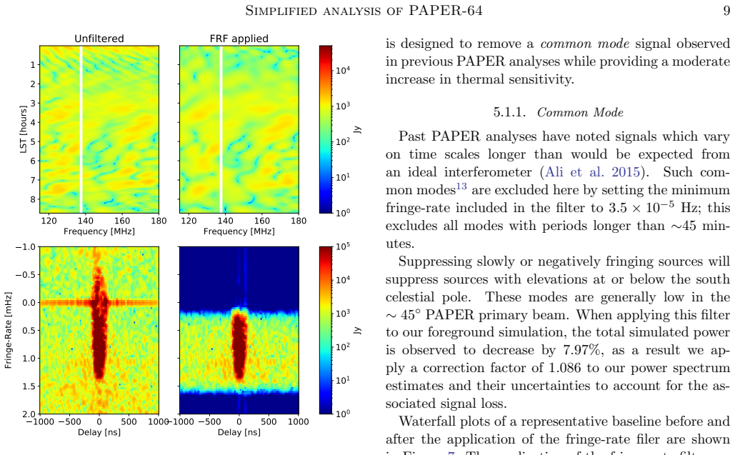
The machinery is the delay-spectrum estimator: visibilities from redundant 30 m baselines are Fourier transformed along frequency with a Blackman-Harris taper, cross-multiplied between baseline pairs and between even/odd day bins, and bootstrap-averaged to form $P(k_\parallel, k_\perp)$ via the paper's Equation 7. A frequency-independent top-hat fringe-rate filter suppresses the zero-fringe-rate common mode, and PRISim foreground simulations set the flux scale and supply the foreground-dependent variance $\sigma_P^2 = 2P_s P_N + P_N^2$. The omission of the delay filter and covariance weighting is the load-bearing simplification that avoids signal loss.
What would settle it
Reprocess the original, uncompressed PAPER-64 visibilities from the correlator output through calibration and LST binning from scratch; if the $z\sim10$ excess at delays $>400$ ns and the imaginary power drop to thermal levels, the upper limits here would not be the limiting uncertainty and the attribution to foregrounds plus non-redundancy would be incomplete.
Extended reading notes
Core claim
The central claim is that when PAPER-64 data are taken through a linear pipeline without foreground filtering or covariance weighting, the statistically significant high-delay power seen in earlier analyses is largely gone; the remaining excess at $|\tau| > 400$ ns tracks foregrounds modulated by LST, baseline non-redundancy, and calibration phase errors, and is not cosmological. The paper therefore reports its results as upper limits, not detections. It further claims, on the basis of signal loss documented in Cheng et al. (2018), that these upper limits supersede all earlier PAPER power spectrum limits, including PAPER-32 results and the PAPER-64 limits of Ali et al. (2015) and Ali et al. (2018).
Load-bearing premise
Everything downstream assumes the archived visibilities---already compressed, redundantly calibrated, absolutely calibrated to Pictor A, and LST-binned by earlier pipelines---are free of spectral or temporal structure injected by those steps; the paper itself states that this compression may imprint systematic biases that it does not investigate.
Editorial extensions
If this is right
- All previous PAPER power spectrum limits are superseded, including PAPER-32 results and the Ali et al. (2015, 2018) PAPER-64 limits.
- Constraints on the intergalactic medium spin temperature that used earlier PAPER upper limits (Pober et al. 2015; Greig et al. 2016) should be disregarded.
- PAPER-64 provides no significant detection of the 21 cm Epoch of Reionization power spectrum; the field's best results remain upper limits.
- Residual high-delay power is attributed to foregrounds and baseline non-redundancy, so future redundant arrays should run redundancy jackknives before cross-multiplying baselines.
- The $z=8.37$ bin analyzed here overlaps the neighboring redshift bins, so its information is not fully independent of the $z=8.13$ and $z=8.68$ bins.
Reading between the lines
- If the archival compression and calibration steps imprinted spectral or temporal structure, the new upper limits could still inherit that bias; re-running from raw visibilities would separate this from sky signals.
- The same simplified estimator could be applied to other redundant arrays: if their high-delay excess also appears mainly in the imaginary cross-power and even-odd null tests, non-redundancy rather than foreground subtraction would be implicated.
- The reported limits sit roughly two orders of magnitude above fiducial reionization models, so they do not yet constrain astrophysics; reaching model levels requires either much longer integrations or removing the non-redundancy noise floor.
- The fitted scale factor of $1.54\pm0.04$ between simulated and observed visibilities hints at a roughly 50 percent amplitude uncertainty in the sky model or calibration; resolving it would tighten the foreground error bars.
Signed reviews
Editorial analysis
A structured set of objections, weighed in public.
Referee Report
Summary. The paper presents a re-analysis of PAPER-64 archival data using a simplified, public power-spectrum pipeline called simpleDS. The analysis deliberately omits several steps that were shown to cause signal loss in earlier PAPER analyses (delay filtering, aggressive fringe-rate filtering, empirical covariance weighting) and uses a uniform FFT-based delay-spectrum estimator. The authors validate the pipeline with a parallel thermal-noise simulation and with PRISim foreground simulations, present multi-redshift power spectra and several null tests, and report 2-sigma upper limits on the 21 cm power spectrum at six redshifts in the range z ~ 7.5 to 10.9. They conclude that high-delay excess power is non-cosmological and that these limits supersede all previous PAPER results.
Significance. If the upper-limit construction is repaired, this would be a valuable contribution. The paper provides an independent, simplified pipeline with publicly available code; the thermal-noise simulation matches the analytic expectation to within about 30%; PRISim is used to check the absolute calibration scale and foreground error bars; and the null tests and imaginary-power diagnostics give a reasonably coherent picture that the high-delay detections are not cosmological. The cautionary message about signal loss in earlier PAPER estimators is important. However, the headline upper limits are not yet statistically valid as stated, and the uninvestigated archival compression and calibration steps weaken the 'lossless' claim.
major comments (3)
- [§9 / Table 2 / Abstract] The headline upper limits are constructed by taking the minimum bandpower over 0.3 < |k| < 0.6 h/Mpc and adding the 2-sigma error of that same band (e.g., Table 2, z=7.49: 5.6e4 + 3.5e4 = 9.1e4 mK^2 ≈ (300 mK)^2; z=9.93: 3.5e6 + 1.9e5 ≈ (1900 mK)^2). Because the selected minimum is an order statistic of many noisy bandpowers, it is biased low relative to a typical bandpower, and adding the selected band's own error does not restore nominal 2-sigma coverage; no trial factor or simultaneous-coverage correction is supplied. The abstract values therefore do not yet have a demonstrated statistical meaning as upper limits. Please report the full Δ²(k) curves and either quote pointwise limits at a pre-specified k with the selection protocol stated, or construct a simultaneous upper limit with an explicit multiplicity correction.
- [§8.2.2 / §9] Section 8.2.2 reports statistically significant even-odd null-test residuals at |τ| > 400 ns in the three highest-redshift bins (Figure 15), yet Section 9 selects the k-range 0.3 < k < 0.6 h/Mpc on the grounds that 'both null-tests pass for most k-modes in each redshift bin.' No quantitative pass criterion is defined, and the selection is made after inspecting the same data that produce the limits. Please specify the metric used to declare a null-test pass, report how many modes pass in each bin, and either exclude failing modes from the limit or propagate the null-test failure into the quoted uncertainty. Without this, the k-range selection is post hoc and the coverage of the quoted limits is unclear.
- [§2.2 / title / abstract] The analysis begins with archival data that were compressed, redundantly calibrated, absolutely calibrated, and LST-binned by earlier pipelines, and the text explicitly states that this compression 'may imprint systematic biases in the data but are not investigated in this work.' Since the paper is titled a 'lossless' re-analysis and the abstract and conclusion state that these limits supersede all previous PAPER results, the uninvestigated pre-pipeline steps are central to the claim. The authors should either investigate the effect of the archival compression and calibration on the final power spectra (for example, by propagating the LST-binning and compression into the simulations used for validation) or clearly qualify in the abstract and conclusions that the new pipeline is lossless only from the calibrated, LST-binned products onward, so inherited systematic biases remain a caveat.
minor comments (6)
- [§2.1] The observing window is given as ending on 'JD 24563745'; this appears to be a typo, likely JD 2456374 or JD 2456374.5.
- [Figure 4 caption] The caption contains 'the there is general agreement'; it should read 'there is general agreement.'
- [§5.1.1] The text has 'suppressed by the the application' and 'fringe-rate filer'; both should be corrected to 'by the application' and 'fringe-rate filter.'
- [§7.1.2] The text refers to 'the nose input described in Section 3'; this should be 'noise input.'
- [§6 / References] The citation 'lglewicz & Hoaglin (1993)' should be 'Iglewicz & Hoaglin (1993)'.
- [§9] The sentence 'These limit supersede all previous PAPER results' should read 'These limits supersede all previous PAPER results.'
Circularity Check
No significant circularity; the quoted 21 cm limits are direct bandpowers from an independent uniform-FFT analysis, not outputs of a fitted model or a self-citation chain.
full rationale
The central upper limits are produced by a uniform-FFT delay transform of calibrated, LST-binned visibilities, cross-multiplication of redundant baseline pairs, and bootstrap variance estimation (Eq. 7; Sections 7 and 9). No parameter fitted to the measured cosmological bandpowers enters the quoted Δ² values. The PRISim scale factor g=1.54 is fit to visibility amplitudes but is used only for foreground error bars and null-test comparisons (Eqs. 9–10; Sections 4.2, 7.1.3, and 8), not for the upper limits themselves, so it is not a fitted input renamed as a prediction. The 1.086 signal-loss correction is derived from the fractional decrease of the foreground simulation under the fringe-rate filter, not from the measured 21 cm power spectrum. The paper's reliance on C18 for the statement that previous PAPER results suffer signal loss and are superseded is a self-citation among overlapping authors, but C18 is external published work, and the present pipeline independently removes the lossy steps (delay filtering, optimal fringe-rate filtering, empirical covariance weighting), so the central derivation does not reduce to that citation. Concerns about the Section 9 choice of the minimum bandpower plus its own 2σ error as an upper limit, and about even-odd null-test residuals at |τ|>400 ns, are statistical-validity and selection-effect issues rather than circularity under the enumerated definitions.
Assumptions & free parameters
free parameters (4)
- PRISim model scale factor g =
1.54 +/- 0.04 (95% confidence)
- Fringe-rate filter low-frequency cutoff =
3.5e-5 Hz
- Signal-loss correction factor =
1.086
- Upper-limit k range =
0.3 < |k| < 0.6 h/Mpc
assumptions (7)
- domain assumption Delay-to-k mapping: baseline length variation over the 10 MHz band is small enough that delay mode tau maps one-to-one to k_parallel (Liu et al. 2014a).
- domain assumption Archival data products (compressed, redundantly calibrated, absolutely calibrated to Pictor A, LST-binned) are unbiased for power spectrum analysis.
- domain assumption The noise model uses Tsys = 180 K * (nu/180 MHz)^-2.55 + 144 K (Rogers & Bowman 2008; C18), with Gaussian, baseline-independent noise.
- domain assumption The PRISim foreground sky model, scaled by g=1.54, adequately represents foreground power for error-bar and null-test interpretation.
- domain assumption The top-hat fringe-rate filter suppresses only common-mode systematics, and the 1.086 correction factor derived from the foreground simulation applies to the cosmological signal as well.
- domain assumption Noise on different baselines is independent, including baselines sharing an antenna, in the variance propagation.
- domain assumption Baselines within each redundant group measure the same sky signal up to thermal noise, after removing antennas 21 and 31.
Cite this review
Pith. "Pith review of A simplified, lossless re-analysis of PAPER-64." pith.science (2026). https://pith.science/paper/LZR7SXA4
@misc{pith2026190902085,
  author       = {Pith},
  title        = {Pith review of: A simplified, lossless re-analysis of PAPER-64},
  year         = {2026},
  howpublished = {\url{https://pith.science/paper/LZR7SXA4}},
  note         = {Machine review of arXiv:1909.02085}
}
abstract
We present limits on the 21cm power spectrum from the Epoch of Reionization (EoR) using data from the 64 antenna configuration of the Donald C. Backer Precision Array for Probing the Epoch of Reionization (PAPER) analyzed through a power spectrum pipeline independent from previous PAPER analyses. Previously reported results from PAPER have been found to contain significant signal loss (Cheng et al. 2018, arxiv:1810.05175). Several lossy steps from previous PAPER pipelines have not been included in this analysis, namely: delay-based foreground filtering, optimal fringe-rate filtering, and empirical covariance-based estimators. Steps which remain in common with previous analyses include redundant calibration and local sidereal time (LST) binning. The power spectra reported here are effectively the result of applying a linear Fourier transform analysis to the calibrated, LST binned data. This analysis also uses more data than previous publications, including the complete available redshift range of $z \sim 7.5$ to $11$. In previous PAPER analyses, many power spectrum measurements were found to be detections of noncosmological power at levels of significance ranging from two to hundreds of times the theoretical noise. Here, excess power is examined using redundancy between baselines and power spectrum jackknives. The upper limits we find on the 21cm power spectrum from reionization are ($1500$ mK)$^{2}$, ($1900$ mK)$^{2}$, ($280$ mK)$^{2}$, ($200$ mK)$^{2}$, ($380$ mK)$^{2}$, ($300$ mK)$^{2}$ at redshifts $z=10.87,\ 9.93,\ 8.68,\ 8.37,\ 8.13,$ and $7.48$, respectively. For reasons described in Cheng et al. 2018 (arxiv:1810.05175), these limits supersede all previous PAPER results (Ali et al. 2018, arxiv:1502.06016).
Figures


Figures from the paper (14 more)




Forward citations
Cited by 5 Pith papers
-
Intensity fluctuations of radio halo in galaxy cluster: Insights from power spectrum estimation
Angular power spectra of 610 MHz radio halos show excess power-law fluctuations only in Abell 2744, requiring multiplicative C_ℓ ∝ ℓ^{-3} structure atop an exponential profile and consistent with ICM turbulence.
-
The EoR 21-cm Bispectrum at $z=8.2$ from MWA data I: Foregrounds and preliminary upper limits
Using 17 minutes of MWA data, the authors place the first comprehensive upper limits on the z=8.2 21-cm bispectrum and characterize its foreground wedge.
-
A Visibility-based 21 cm Bispectrum Estimator for Radio-interferometric Data
A gridded-visibility, FFT-accelerated estimator for the binned 21 cm multi-frequency angular bispectrum and 3D bispectrum is presented and validated against simulations with an input bispectrum model.
-
A visibility-based angular bispectrum estimator for radio-interferometric data
An FFT-based estimator recovers the angular bispectrum from gridded radio-interferometric visibilities across all triangle shapes, validated on simulated MWA data at 154.25 MHz.
-
Investigating radio source population $\&$ spatial characteristics of diffuse Galactic synchrotron emission in the GAMA-23 field with uGMRT Band-3
A 325 MHz uGMRT mosaic of the GAMA-23 field yields a 5741-source catalog, source counts, spectral indices, and angular power spectra of diffuse Galactic synchrotron emission.
Reference graph
Works this paper leans on
-
[2]
Ali, Z. S., Parsons, A. R., Zheng, H., et al. 2015, ApJ, 809, 61, doi: 10.1088/0004-637X/809/1/61 —. 2018, ApJ, 863, 201, doi: 10.3847/1538-4357/aad7b4
-
[3]
Andrae, R. 2010, ArXiv e-prints. https://arxiv.org/abs/1009.2755 Astropy Collaboration, Robitaille, T. P., Tollerud, E. J., et al. 2013, aap, 558, A33, doi: 10.1051/0004-6361/201322068
arXiv 2010
-
[4]
2001, PhR, 349, 125, doi: 10.1016/S0370-1573(01)00019-9 —
Barkana, R., & Loeb, A. 2001, PhR, 349, 125, doi: 10.1016/S0370-1573(01)00019-9 —. 2007, Reports on Progress in Physics, 70, 627, doi: 10.1088/0034-4885/70/4/R02 26 Kolopanis et al
-
[5]
Beardsley, A. P., Hazelton, B. J., Sullivan, I. S., et al. 2016, ApJ, 833, 102, doi: 10.3847/1538-4357/833/1/102
-
[6]
Bernardi, G., de Bruyn, A. G., Brentjens, M. A., et al. 2009, A&A, 500, 965, doi: 10.1051/0004-6361/200911627
-
[7]
Bernardi, G., de Bruyn, A. G., Harker, G., et al. 2010, A&A, 522, A67+, doi: 10.1051/0004-6361/200913420
-
[8]
Bernardi, G., Greenhill, L. J., Mitchell, D. A., et al. 2013, ApJ, 771, 105, doi: 10.1088/0004-637X/771/2/105
-
[9]
Bernardi, G., Zwart, J. T. L., Price, D., et al. 2016, MNRAS, 461, 2847, doi: 10.1093/mnras/stw1499
Show all 67 references
-
[10]
D., & Rogers, A
Bowman, J. D., & Rogers, A. E. E. 2010, Nature, 468, 796, doi: 10.1038/nature09601
2010 doi
-
[11]
R., Kolopanis, M., et al
Cheng, C., Parsons, A. R., Kolopanis, M., et al. 2018, ApJ, 868, 26, doi: 10.3847/1538-4357/aae833
2018 doi
-
[12]
Clark, B. G. 1999, in Astronomical Society of the Pacific Conference Series, Vol. 180, Synthesis Imaging in Radio Astronomy II, ed. G. B. Taylor, C. L. Carilli, & R. A. Perley, 1–+
1999
-
[13]
D., Condon, J
Cotton, W. D., Condon, J. J., Perley, R. A., et al. 2004, in Society of Photo-Optical Instrumentation Engineers (SPIE) Conference Series, Vol. 5489, Ground-based Telescopes, ed. J. Oschmann, Jacobus M., 180–189 de Oliveira-Costa, A., Tegmark, M., Gaensler, B. M., et al. 2008, ...
2004
-
[14]
R., Parsons, A
DeBoer, D. R., Parsons, A. R., Aguirre, J. E., et al. 2016, ArXiv e-prints. https://arxiv.org/abs/1606.07473
2016 arXiv
-
[15]
S., Liu, A., Williams, C
Dillon, J. S., Liu, A., Williams, C. L., et al. 2014, PhRvD, 89, 023002, doi: 10.1103/PhysRevD.89.023002
2014 doi
-
[16]
S., Neben, A
Dillon, J. S., Neben, A. R., Hewitt, J. N., et al. 2015, Phys. Rev. D, 91, 123011, doi: 10.1103/PhysRevD.91.123011
2015 doi
-
[17]
S., Kohn, S
Dillon, J. S., Kohn, S. A., Parsons, A. R., et al. 2018, MNRAS, 477, 5670, doi: 10.1093/mnras/sty1060
2018 doi
-
[18]
1994, An Introduction to the
Efron, B., & Tibshirani, R. 1994, An Introduction to the
1994
-
[19]
R., Oh, S
Furlanetto, S. R., Oh, S. P., & Briggs, F. H. 2006, PhR, 433, 181, doi: 10.1016/j.physrep.2006.08.002
2006 doi
-
[20]
S., & Chengalur, J
Ghosh, A., Bharadwaj, S., Ali, S. S., & Chengalur, J. N. 2011, MNRAS, 418, 2584, doi: 10.1111/j.1365-2966.2011.19649.x G´ orski, K. M., Hivon, E., Banday, A. J., et al. 2005, ApJ, 622, 759, doi: 10.1086/427976
2011
-
[21]
Greig, B., Mesinger, A., & Pober, J. C. 2016, MNRAS, 455, 4295, doi: 10.1093/mnras/stv2618
2016 doi
-
[22]
2017, HERA-Team/pyuvdata: Version 1.2, doi: 10.5281/zenodo.1044022
Hazelton, B., Beardsley, A., Pober, J., et al. 2017, HERA-Team/pyuvdata: Version 1.2, doi: 10.5281/zenodo.1044022. https://doi.org/10.5281/zenodo.1044022 H¨ ogbom, J. A. 1974, A&AS, 15, 417
2017 doi
-
[23]
R., Hancock, P
Hurley-Walker, N., Callingham, J. R., Hancock, P. J., et al. 2017, MNRAS, 464, 1146, doi: 10.1093/mnras/stw2337
2017 doi
-
[24]
T., van der Tol, S., Cotton, W
Intema, H. T., van der Tol, S., Cotton, W. D., et al. 2009, A&A, 501, 1185, doi: 10.1051/0004-6361/200811094
2009 doi
-
[25]
C., Parsons, A
Jacobs, D. C., Parsons, A. R., Aguirre, J. E., et al. 2013, ApJ, 776, 108, doi: 10.1088/0004-637X/776/2/108
2013 doi
-
[26]
C., Pober, J
Jacobs, D. C., Pober, J. C., Parsons, A. R., et al. 2015, ApJ, 801, 51, doi: 10.1088/0004-637X/801/1/51
2015 doi
-
[27]
C., Hazelton, B
Jacobs, D. C., Hazelton, B. J., Trott, C. M., et al. 2016, ApJ, 825, 114, doi: 10.3847/0004-637X/825/2/114
2016 doi
-
[28]
2001–, SciPy: Open source scientific tools for Python
Jones, E., Oliphant, T., Peterson, P., et al. 2001–, SciPy: Open source scientific tools for Python. http://www.scipy.org/
2001
-
[29]
C., Trott, C
Joseph, R. C., Trott, C. M., & Wayth, R. B. 2018, AJ, 156, 285, doi: 10.3847/1538-3881/aaec0b
2018 doi
-
[30]
R., Pober, J
Kerrigan, J. R., Pober, J. C., Ali, Z. S., et al. 2018, ApJ, 864, 131, doi: 10.3847/1538-4357/aad8bb lglewicz, B., & Hoaglin, D. C. 1993, Volume 16: How to Detect and Handle Outliers, ed. P. Edward F. Mykytka (The ASQC Basic References in Quality Control: Statistical Techniques)
2018 doi
-
[31]
Liu, A., & Parsons, A. R. 2016, MNRAS, 457, 1864, doi: 10.1093/mnras/stw071
2016 doi
-
[32]
R., & Trott, C
Liu, A., Parsons, A. R., & Trott, C. M. 2014a, Phys. Rev. D, 90, 023018, doi: 10.1103/PhysRevD.90.023018 —. 2014b, Phys. Rev. D, 90, 023019, doi: 10.1103/PhysRevD.90.023019
-
[34]
Loeb, A., & Furlanetto, S. R. 2013, The First Galaxies in the Universe (Princeton University Press)
2013
-
[35]
2015, MNRAS, 446, 3478, doi: 10.1093/mnras/stu2310
McKinley, B., Yang, R., L´ opez-Caniego, M., et al. 2015, MNRAS, 446, 3478, doi: 10.1093/mnras/stu2310
2015 doi
-
[36]
2007, in Astronomical Society of the Pacific Conference Series, Vol
Golap, K. 2007, in Astronomical Society of the Pacific Conference Series, Vol. 376, Astronomical Data Analysis Software and Systems XVI, ed. R. A. Shaw, F. Hill, & D. J. Bell, 127
2007
-
[37]
Mellema, G., Koopmans, L. V. E., Abdalla, F. A., et al. 2013, Experimental Astronomy, 36, 235, doi: 10.1007/s10686-013-9334-5
2013 doi
-
[38]
2011, MNRAS, 411, 955, doi: 10.1111/j.1365-2966.2010.17731.x
Mesinger, A., Furlanetto, S., & Cen, R. 2011, MNRAS, 411, 955, doi: 10.1111/j.1365-2966.2010.17731.x
2011
-
[39]
F., Aguirre, J
Moore, D. F., Aguirre, J. E., Kohn, S. A., et al. 2017, ApJ, 836, 154, doi: 10.3847/1538-4357/836/2/154
2017 doi
-
[40]
F., & Wyithe, J
Morales, M. F., & Wyithe, J. S. B. 2010, ARA&A, 48, 127, doi: 10.1146/annurev-astro-081309-130936 Simplified analysis of PAPER-64 27
2010 doi
-
[41]
Jones, M. E. 2010, in Phased Array Systems and Technology (ARRAY), 2010 IEEE International Symposium on, IEEE, 690–694
2010
-
[42]
Oh, S. P. 2001, ApJ, 553, 499, doi: 10.1086/320957
2001 doi
-
[43]
2006–, NumPy: A guide to NumPy, USA: Trelgol Publishing
Oliphant, T. 2006–, NumPy: A guide to NumPy, USA: Trelgol Publishing. http://www.numpy.org/
2006
-
[44]
G., Bandura, K., et al
Paciga, G., Albert, J. G., Bandura, K., et al. 2013, MNRAS, 433, 639, doi: 10.1093/mnras/stt753
2013 doi
-
[45]
2012a, ApJ, 753, 81, doi: 10.1088/0004-637X/753/1/81
Aguirre, J. 2012a, ApJ, 753, 81, doi: 10.1088/0004-637X/753/1/81
-
[46]
R., & Backer, D
Parsons, A. R., & Backer, D. C. 2009, AJ, 138, 219, doi: 10.1088/0004-6256/138/1/219
2009 doi
-
[47]
R., Liu, A., Ali, Z
Parsons, A. R., Liu, A., Ali, Z. S., & Cheng, C. 2016, ApJ, 820, 51, doi: 10.3847/0004-637X/820/1/51
2016 doi
-
[48]
R., Pober, J
Parsons, A. R., Pober, J. C., Aguirre, J. E., et al. 2012b, ApJ, 756, 165, doi: 10.1088/0004-637X/756/2/165
-
[49]
R., Backer, D
Parsons, A. R., Backer, D. C., Foster, G. S., et al. 2010, AJ, 139, 1468, doi: 10.1088/0004-6256/139/4/1468
2010 doi
-
[50]
R., Liu, A., Aguirre, J
Parsons, A. R., Liu, A., Aguirre, J. E., et al. 2014, ApJ, 788, 106, doi: 10.1088/0004-637X/788/2/106
2014 doi
-
[51]
H., Yatawatta, S., Koopmans, L
Patil, A. H., Yatawatta, S., Koopmans, L. V. E., et al. 2017, ApJ, 838, 65, doi: 10.3847/1538-4357/aa63e7
2017 doi
-
[52]
2015, ApJ, 801, 138, doi: 10.1088/0004-637X/801/2/138
Patra, N., Subrahmanyan, R., Sethi, S., Udaya Shankar, N., & Raghunathan, A. 2015, ApJ, 801, 138, doi: 10.1088/0004-637X/801/2/138
2015 doi
-
[53]
C., Parsons, A
Pober, J. C., Parsons, A. R., Jacobs, D. C., et al. 2012, AJ, 143, 53, doi: 10.1088/0004-6256/143/2/53
2012 doi
-
[54]
C., Parsons, A
Pober, J. C., Parsons, A. R., Aguirre, J. E., et al. 2013, ApJL, 768, L36, doi: 10.1088/2041-8205/768/2/L36
2013 doi
-
[55]
C., Liu, A., Dillon, J
Pober, J. C., Liu, A., Dillon, J. S., et al. 2014, ApJ, 782, 66, doi: 10.1088/0004-637X/782/2/66
2014 doi
-
[56]
C., Ali, Z
Pober, J. C., Ali, Z. S., Parsons, A. R., et al. 2015, ApJ, 809, 62, doi: 10.1088/0004-637X/809/1/62
2015 doi
-
[57]
C., Hazelton, B
Pober, J. C., Hazelton, B. J., Beardsley, A. P., et al. 2016, ApJ, 819, 8, doi: 10.3847/0004-637X/819/1/8
2016 doi
-
[58]
R., & Loeb, A
Pritchard, J. R., & Loeb, A. 2010, PhRvD, 82, 023006, doi: 10.1103/PhysRevD.82.023006
2010 doi
-
[59]
Rogers, A. E. E., & Bowman, J. D. 2008, AJ, 136, 641, doi: 10.1088/0004-6256/136/2/641
2008 doi
-
[60]
G., Cooray, A., & Knox, L
Santos, M. G., Cooray, A., & Knox, L. 2005, ApJ, 625, 575, doi: 10.1086/429857
2005 doi
-
[61]
E., Wayth, R
Sokolowski, M., Tremblay, S. E., Wayth, R. B., et al. 2015, PASA, 32, 4, doi: 10.1017/pasa.2015.3
2015 doi
-
[62]
S., Morales, M
Sullivan, I. S., Morales, M. F., Hazelton, B. J., et al. 2012, ApJ, 759, 17, doi: 10.1088/0004-637X/759/1/17
2012 doi
-
[63]
2019, PRISim: Precision Radio Interferometry Simulator (for radio astronomy applications), 0.2-alpha, Zenodo, doi: 10.5281/zenodo.2548117
Thyagarajan, N., Kolopanis, M., Jacobs, D., Murray, S., & santoshmh. 2019, PRISim: Precision Radio Interferometry Simulator (for radio astronomy applications), 0.2-alpha, Zenodo, doi: 10.5281/zenodo.2548117. https://doi.org/10.5281/zenodo.2548117
2019 doi
-
[64]
C., Bowman, J
Thyagarajan, N., Jacobs, D. C., Bowman, J. D., et al. 2015a, ApJL, 807, L28, doi: 10.1088/2041-8205/807/2/L28 —. 2015b, ApJ, 804, 14, doi: 10.1088/0004-637X/804/1/14
-
[65]
J., Goeke, R., Bowman, J
Tingay, S. J., Goeke, R., Bowman, J. D., et al. 2013, PASA, 30, 7, doi: 10.1017/pasa.2012.007
2013 doi
-
[66]
B., & L´ opez-Cruz, O
Peterson, J. B., & L´ opez-Cruz, O. 2014, ApJL, 782, L9, doi: 10.1088/2041-8205/782/1/L9
2014 doi
-
[67]
B., Lenc, E., Bell, M
Wayth, R. B., Lenc, E., Bell, M. E., et al. 2015, PASA, 32, e025, doi: 10.1017/pasa.2015.26
2015 doi
-
[68]
G., Brentjens, M
Yatawatta, S., de Bruyn, A. G., Brentjens, M. A., et al. 2013, A&A, 550, A136, doi: 10.1051/0004-6361/201220874
2013 doi
-
[69]
2014, MNRAS, 445, 1084, doi: 10.1093/mnras/stu1773 APPENDIX A
Zheng, H., Tegmark, M., Buza, V., et al. 2014, MNRAS, 445, 1084, doi: 10.1093/mnras/stu1773 APPENDIX A. FOREGROUND DEPENDENT VARIANCE To find the variance of P (k), being by assuming each visibility ˜Vi(τ,u,v,w ) = s +ni is the sum of the true sky signal, s , and a noise compon...
2014 doi
Reviewed August 14, 2026 · model on record in the stance chip above.
Discussion (0). Continue with ORCID to comment.