Inductive-bias-driven Reinforcement Learning For Efficient Schedules in Heterogeneous Clusters

Ravishankar K. Iyer; Saurabh Jha; Subho S Banerjee; Zbigniew T. Kalbarczyk

REVIEW 5 major objections 5 minor 12 references

Inductive-bias-driven Reinforcement Learning For Efficient Schedules in Heterogeneous Clusters

T0 review · 5 major / 5 minor · reviewed 2026-08-14 · deepseek-v4-flash

Challenge this review Re-run · record.json Download PDF Read on arXiv ↗ Review JSON

Pith's one-line read This paper claims that scheduling on heterogeneous clusters can be learned sample-efficiently by encoding the machine's own architecture as a Bayesian network, cutting average job completion time by up to 32% over hand-tuned heuristics…

desk verdict A real system with credible scheduling results, but the key 'no-inference' gradient claim is underspecified and the training-time comparison is confounded. read the letter →

arxiv 1909.02119 v2 pith:BPQ2I7N2 submitted 2019-09-04 cs.DC cs.LG

Subho S Banerjee , Saurabh Jha , Zbigniew T. Kalbarczyk , Ravishankar K. Iyer This is my paper · ORCID

classification cs.DCcs.LG

keywords heterogeneousschedulingBayesianreinforcementlearningPOMDPperformancecountersinductivebiassampling-basedgradientsdatacenterGPU-FPGAaccelerators

verification ladder T0 review T1 audit T2 compute T3 formal

The pith

A machine-rendered reading of the paper's core claim, the machinery that carries it, and where it could break.

The reading

This paper proposes Symphony, a scheduler that treats the scheduling problem as a partially observable Markov decision process and injects architectural domain knowledge as a Bayesian network, so an RL agent can infer hidden resource utilization, such as PCIe bandwidth, from performance-counter readings. The paper claims this inductive bias makes training far more sample-efficient than black-box RL, and that a sampling-based gradient estimator removes the need for full Bayesian inference during training. On a rack-scale heterogeneous testbed with CPUs, GPUs, and FPGAs, Symphony is reported to reduce average job completion time by up to 32% compared to hand-tuned heuristics and to come within 6% of an oracle schedule, while training about 4x faster than full Bayesian inference and about 2.2x faster than black-box ML. A sympathetic reader should care because schedulers for accelerator-rich data centers currently rely on case-by-case heuristics, and this is a concrete attempt to replace heuristic search with a reusable, domain-structured learning procedure.

What carries the argument

The central object is a Bayesian network over system state, constructed from processor documentation, whose nodes are performance-counter measurements and hidden resource utilizations, connected according to known microarchitectural and topology relationships. Inference on this network produces the POMDP belief state that feeds the policy and value networks. The load-bearing mechanism is a sampling-based gradient estimator that replaces full Bayesian inference during backpropagation: it draws samples from the network's conditional distributions and uses frequency counts to estimate gradient terms, making training tractable for polytree networks and decoupling BN training from the inference procedure used at decision time.

What would settle it

Measure the actual utilization of a hidden resource, such as PCIe link bandwidth, using direct instrumentation on a testbed, run the BN inference on concurrent performance-counter samples, and compare the two; if the BN's posterior estimate diverges systematically from measured utilization in regimes where scheduling decisions matter, the claimed sample-efficiency advantage of Symphony would not survive on that platform.

Watch

Extended reading notes

Core claim

The paper's central claim is that a scheduling policy can be learned from far fewer workload executions if the learning agent is given a model of the machine's hidden resource dependencies rather than having to discover them from data. In Symphony, this inductive bias is a Bayesian network over performance-counter measurements; processor manuals supply deterministic algebraic relationships between counters and resource utilizations, and inference on this network yields a belief state used by a graph-network-and-LSTM policy. The paper further claims that the gradient of this Bayesian model can be approximated by sampling from the network's causal structure, avoiding full probabilistic inference at every training step, which removes a known obstacle to using deep Bayesian RL in dynamic real-world deployments. The evaluation on real genomics, EEG, and security workloads is the evidence that the bias pays off: better schedules with less training.

Load-bearing premise

The load-bearing premise is that the hand-built Bayesian network in Figure 5 correctly captures how performance-counter measurements relate to the hidden resource utilizations that actually determine performance; the paper does not validate those latent estimates against ground truth.

Editorial extensions

If this is right

Because the Bayesian network is rebuilt only when the underlying hardware configuration changes, roughly every five to six years as the paper notes, Symphony can absorb new accelerators without a from-scratch retraining campaign.
The sampling-based gradient estimator makes periodic retraining of a scheduling policy practical in a data center, since training no longer requires full probabilistic inference at every step.
The same POMDP-plus-Bayesian-network structure should transfer to any scheduling domain where a hidden shared resource creates contention, such as network or co-flow scheduling, without requiring a new hand-tuned heuristic.
On the evaluated workloads, the resulting schedules come within 6% of the oracle at the 99th percentile, meaning the gap between learned and optimal scheduling shrinks to near-noise levels.

Reading between the lines

Editorial extensions of the paper, not claims the author makes directly.

I infer that the accuracy of the BN's latent resource estimates is the decisive factor: if those estimates are wrong, the inductive bias could actively mislead the policy, and the sample-efficiency advantage would vanish.
I infer the method could be stress-tested by replacing the hand-built BN with a randomly structured or learned graph; if the graph structure itself, rather than the sampling gradient trick, drives the gains, then the cost of manual BN construction remains the key barrier.
I infer that validation against direct hardware measurement, for example comparing inferred PCIe utilization with link-level counters, would be a natural next test that the paper does not report.

Share X Bluesky LinkedIn Reddit HN

Signed reviews

No signed human review yet.

Editorial analysis

A structured set of objections, weighed in public.

Desk editor's note, referee report, and a circularity audit.

Desk Editor's Note

read the letter

Simon, you asked about Symphony. Here's my take, which mostly tracks the reader's report: there's a real system here with a credible empirical evaluation, but the main algorithmic claim is overstated.

The genuinely new piece is the use of a domain-driven Bayesian network as an inductive bias for an RL scheduler, with the BN built from processor manuals and OS counter definitions. That is a nice idea, and the graph-network encoding of system topology plus the DFG is a sensible design. The scheduling experiments are also credible: 500 executions, three real workloads, and a hand-computed exhaustive oracle. The 32% improvement over Paragon and 6% gap to oracle are the kind of numbers that would make a datacenter operator pay attention.

Now the soft spots, in order of size. The biggest is the gradient estimator in Section 3. Equations 2 through 5 require samples from conditional distributions of the form Pr(parents | evidence). The paper says only forward sampling is needed, but the evidence is continuous performance-counter values modeled with t-distributions. Naive forward sampling cannot condition on a continuous observation; you need MCMC, likelihood weighting, or something similar. The paper never explains how those conditional samples are drawn. The evaluation section implicitly concedes this: 'All Opt' uses the FPGA 'for BN inference,' citing the authors' own MCMC accelerator. So the 4.3x training-time improvement is not inference-free versus inference-based; it is one approximate inference scheme versus another. The complexity analysis in Section 3.1 omits the sampling cost entirely. This is a load-bearing problem for the paper's central claim.

The scheduling results themselves are less affected, because the deployed policy uses BN inference to compute belief states, and the performance is measured after training. So the empirical story probably survives, but the 'no inference' contribution needs to be either corrected or re-scoped. Second, the reward function description (rt = -sum 1/T_i) is confusingly worded and should be cleaned up. Third, there are no error bars on the key figures, which is a shame given 500 runs. No released artifacts either, but that is common in this subfield and not a deal-breaker. The self-citations to the FPGA accelerator are relevant because the hardware is actually used; citing your own prior work for a component you built is not a flaw.

Who should read this? Systems people working on ML-driven scheduling, and anyone interested in inductive biases for RL. It deserves a serious referee; I would send it out, but with a request to either specify the sampling mechanism and redo the training-time comparison, or clearly scope the contribution as 'approximate inference via sampling' rather than 'no inference.'

Referee Report

5 major / 5 minor

Summary. The paper proposes Symphony, a scheduling framework for heterogeneous CPU/GPU/FPGA clusters that combines a domain-driven Bayesian network (BN) for resource-utilization estimation with an actor-critic RL policy, and a sampling-based gradient estimator that supposedly computes BN gradients without full probabilistic inference. The central claims are that this inductive bias reduces training data and training time relative to black-box RL, that the resulting scheduler improves average job completion time by up to 32% over hand-tuned baselines and comes within 6% of an oracle, and that the sampling-based gradient method is about 4.3x more training-efficient than belief-propagation-based training and about 2.2x faster than black-box RL. The evaluation is performed on a rack-scale cluster of Power8 CPUs, K40/K80 GPUs, and FPGAs using three real workloads.

Significance. If the gradient-estimation mechanism is correct, the paper makes a useful contribution: it offers a concrete recipe for injecting architectural knowledge into RL for scheduling while avoiding per-step posterior inference, and it demonstrates nontrivial improvements on a real heterogeneous testbed. The paper also deserves credit for evaluating on physical hardware with multiple accelerators, for using an exhaustive schedule search as an oracle baseline, and for exposing a real PCIe contention effect (Fig. 1) that motivates the need for fine-grained resource modeling. However, the significance is conditional on the correctness and feasibility of the claimed inference-free gradient computation, which is the paper's main technical novelty, and that mechanism is currently underspecified.

major comments (5)

[Section 3, Eqns. (2)-(5)] The sampling-based gradient estimator is underspecified in a way that is load-bearing for the central 'no-inference' claim. Equations (2), (3), and (5) require samples from conditional distributions of the form Pr(℘(X)=y | ξ=a) and Pr(N=n | ξ=a), where ξ is an observed ancestor. The paper never explains how these conditional samples are generated. If the samples are drawn by rejection sampling from the joint, then for continuous evidence ξ=a, which the BN models with t-distributions on performance-counter values (Section 4, BN Model), the probability of drawing an exact match is zero; some approximate-inference procedure such as likelihood weighting, particle filtering, or MCMC is required. If such a procedure is used, then the statement in Section 2 that gradients are computed 'without requiring computation of full Bayesian inference' is misleading, and the 4.3x training-time comparison in Fig. 10 is no longer a clean comparison between inference-free and inference-based training. The authors need to state exactly what conditional-sampling algorithm is used, provide its cost, and either remove the 'no inference' claim or qualify it precisely.
[Section 3.1, Computational Complexity] The complexity analysis reports O(S) for Eqns. (2) and (3) and O(mS) for Eqn. (5), but it treats the conditional samples n_S(a, y_i) and n_S(a, n_k) as free. The cost of producing S samples satisfying the conditioning event ξ=a must be included in the total. For continuous evidence, the acceptance rate of any exact rejection scheme is zero, and even for discrete evidence the cost scales with the inverse of the conditioning probability. As written, the claimed complexity advantage over posterior inference is not established. The authors should either give the sampling algorithm and its sample-generation cost, or revise the complexity claim to include it.
[Section 4, BN Model and Fig. 5] The paper provides no validation of the BN's inferred resource-utilization values against ground truth. The entire sample-efficiency argument rests on the premise that the hand-built BN, constructed from processor manuals, correctly captures the statistical relationship between performance counters and hidden resource utilizations. If this mapping is wrong, the inductive bias misleads the RL agent and the reported training-time gains disappear. I would like to see a direct evaluation of the BN's latent estimates against measurable ground truth on at least a subset of resources, or an ablation in which BN edges are randomly rewired to show that the specific structure matters. Without such evidence, the causal role of the inductive bias in the reported gains is not established.
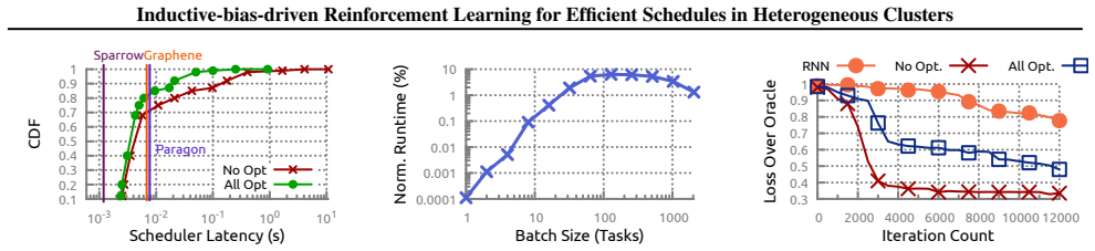
[Section 5, State of the Art and Fig. 6] The comparison against baselines is weakened by the fact that the paper itself argues Paragon, Graphene, and Sparrow are not well-suited to heterogeneous accelerator-rich systems, and the supplementary material states that Graphene was modified for the heterogeneous setting. Since the headline result (32% improvement over the second-best baseline) depends on these baselines' performance, the comparison should include either an unmodified baseline, a description of the exact modifications and their impact, or an additional heterogeneous-aware baseline such as a tuned heuristic or a recent heterogeneity-aware scheduler. As written, the reader cannot tell how much of the measured advantage comes from the method and how much from the baselines being evaluated in conditions they were not designed for.
[Section 5, Training Time (Fig. 10)] The 'All Opt' configuration, which is credited with the 4.3x training-time improvement, includes an FPGA accelerator for BN inference and task batching, while the 'No Opt' configuration does not appear to use those accelerations. This confounds the algorithmic contribution of the sampling-based gradient method with hardware acceleration and batching. The training-time comparison should separate these factors, e.g., by comparing the sampling-based gradient method against belief propagation with both configurations using the same hardware, so the claimed improvement can be attributed to the gradient estimator rather than to the FPGA and batching.

minor comments (5)

[Abstract and Section 5] The abstract states 'up to 2.2x' for training-time improvement over black-box approaches, while the introduction and Section 5 report a 4x/4.3x improvement over full Bayesian inference and a 2.2x improvement over the RNN baseline; the numbers should be reconciled and labeled as wall-clock time or sample-efficiency consistently.
[Section 5, Fig. 8] The caption for Fig. 8 says the tail latency is 100x larger than the median and that batching reduces tail latency by 12x, but the reference to 'see Fig. 3' appears to be a typo; it should reference Fig. 9 where the batch-size experiment is shown.
[Section 3, Eqns. (2)-(5)] The notation n_S(a, n_k) and n_S(y_i, a, n_k) is introduced without a definition; the earlier definition n_S(j) counts occurrences of value j in a sample set, and the conditional variants need to be defined explicitly.
[Section 4, Reward Function] The reward r_t = -∑_{i=0}^{t} 1/T_i is described as representing makespan, but the formula as written is a cumulative sum over actions; the precise relationship to makespan and how parallel actions are not double-counted should be stated more formally.
[Section 5, Fig. 10] Fig. 10 shows learning curves without error bars or multiple-seed variation; given the small number of parallel environments (n_e=2) and the stochasticity of RL training, reporting variance across seeds would make the 2.2x and 4.3x claims more convincing.

Circularity Check

1 steps flagged · score 6.0 of 10

The 'inference-free' gradient estimator is defined in terms of conditional samples that are themselves the output of Bayesian inference.

self definitional [Section 3.1, Eqns. (2)-(5); Section 2 'Reducing Training Time'; Section 4 'BN Model']
"The key is to calculate the gradient by generating samples from the model, which is computationally simpler than inferring the posterior distribution. ... All that is required is the ability to generate samples from the BN. ... ≈ S∑ i=1 nS(a, yi) nS(a) ∂fX(x, yi; θX) ∂θX ."

Eq. (2) is a Monte Carlo replacement for the integral over Pr(℘(X)=y|ξ=a), and nS(a,yi)/nS(a) is exactly the empirical conditional distribution of the parents ℘(X) given evidence ξ=a. Producing samples from that conditional distribution is the inference operation the paper claims to avoid; for the continuous performance-counter evidence modeled with t-distributions in §4, exact equality events have probability zero, so ancestral sampling from the joint cannot supply the samples, and any workable mechanism (likelihood weighting, MCMC, particle filtering) is approximate inference. The 'samples from the BN' used as input are therefore already the output of Bayesian inference, making the claimed inference-free gradient computation self-definitional.

full rationale

The end-to-end scheduling evaluation (Figs. 6-9) is self-contained: Symphony is benchmarked against external schedulers (Paragon, Graphene, Sparrow) and an exhaustive oracle, so the 32%/6% job-completion-time claims are not circular. The BN parameters are fitted to the testbed, but the evaluation compares fitted-system performance against external baselines rather than renaming a fitted quantity as a prediction. The self-citation to the FPGA accelerator (Banerjee et al. 2019b) is a tooling dependency, not a load-bearing circular argument. The genuine circular/definitional problem is in the training-time contribution: the gradient equations in §3.1 use posterior conditional sample counts nS(a,yi)/nS(a), so the proposed 'without full Bayesian inference' algorithm is defined in terms of inference outputs. That makes the headline training-time advantage partially circular, though not the scheduling-quality results; hence score 6 rather than 8 or 10. I do not score the separate issue that 'All Opt' also bundles task batching and FPGA inference into the 4.3x comparison, since that is a confounding/attribution problem rather than a by-construction circularity.

Assumptions & free parameters 4 free parameters · 5 assumptions · 0 invented entities

The central claim rests on the correctness of the hand-built Bayesian network, the availability of kernel implementations, and the accuracy of the sampling-based gradient estimator. The BN's structure is assumed correct without ground-truth validation; the gradient estimator's convergence is not proven.

free parameters (4)

theta_MB (memory bandwidth stall threshold) = not specified (learned when unknown)
Used in the PC composition to compute memory bandwidth utilization; the paper states it is processor-specific and learned via training when unknown (Section 4, BN Model).
BN conditional parameters Theta_BN = learned during training
The conditional distributions of the Bayesian network over resource utilization, including thresholds and statistical relationships, are trained from system measurements and the RL loss.
Measurement noise variance sigma = estimated from sample variance
The noise model e_c ~ N(0,sigma) with unknown sigma; the paper uses sample variance to form a t-distribution, so sigma is not given a priori.
A3C hyperparameters (learning rate, LSTM unroll, n_s, n_e) = learning rate 0.005, unroll 20, n_s=20, n_e=2
Chosen by hand; listed in Table 3 of the supplementary material.

assumptions (5)

domain assumption The BN graph structure in Fig. 5 correctly represents the causal/statistical relationships between performance counters and hidden resource utilizations.
The entire inductive bias is built on this manually constructed graph; no validation against ground-truth utilizations is provided.
domain assumption Algebraic relationships from processor manuals can be encoded as differentiable diffeomorphisms (Section 3.1).
The gradient derivation for deterministic nodes requires this differentiability; not all hardware formulas may be diffeomorphic.
domain assumption Measurement errors are Gaussian with zero systematic error (Section 4, BN Model).
Based on prior work (Weaver & McKee 2008); if systematic errors exist, the belief state is biased.
ad hoc to paper The sampling-based gradient estimates in Eqns 2-5 are accurate enough for training; the paper provides no bias/variance analysis.
The recursive Monte Carlo estimator may be biased in finite samples; convergence is not proven.
domain assumption Kernels are known ahead of time and have multiple implementations for different processors (Section 4, Workload & Programming Model).
The scheduler chooses among known kernel implementations; if kernels change, the model must be retrained.

how reviews work

0 comments

Cite this review

Pith. "Pith review of Inductive-bias-driven Reinforcement Learning For Efficient Schedules in Heterogeneous Clusters." pith.science (2026). https://pith.science/paper/BPQ2I7N2

@misc{pith2026190902119,
  author       = {Pith},
  title        = {Pith review of: Inductive-bias-driven Reinforcement Learning For Efficient Schedules in Heterogeneous Clusters},
  year         = {2026},
  howpublished = {\url{https://pith.science/paper/BPQ2I7N2}},
  note         = {Machine review of arXiv:1909.02119}
}

read the original abstract

The problem of scheduling of workloads onto heterogeneous processors (e.g., CPUs, GPUs, FPGAs) is of fundamental importance in modern data centers. Current system schedulers rely on application/system-specific heuristics that have to be built on a case-by-case basis. Recent work has demonstrated ML techniques for automating the heuristic search by using black-box approaches which require significant training data and time, which make them challenging to use in practice. This paper presents Symphony, a scheduling framework that addresses the challenge in two ways: (i) a domain-driven Bayesian reinforcement learning (RL) model for scheduling, which inherently models the resource dependencies identified from the system architecture; and (ii) a sampling-based technique to compute the gradients of a Bayesian model without performing full probabilistic inference. Together, these techniques reduce both the amount of training data and the time required to produce scheduling policies that significantly outperform black-box approaches by up to 2.2x.

Figures

Figures reproduced from arXiv: 1909.02119 by the authors.

**Figure 1.** Performance degradation due to PCIe contention between GPU and NIC (averaged over 10 runs). et al., 1997). It is this cost that makes the use of deep RL techniques in dynamic real-world deployments (which require periodic retraining) prohibitively expensive. To address that issue, we have developed a procedure for computing the gradient of variables in the above Bayesian model without requiring full inference com… view at source ↗

**Figure 2.** The proposed RL architecture. parameters ΘBN ). A BN is a probabilistic graphical model that represents a set of variables and their conditional dependencies via a directed acyclic graph (DAG). We use probabilistic inference on the BN to calculate an estimate of the belief state ˆbt. ˆbt is then used in an NN fπ( ˆbt; Θπ) (with parameters Θπ) to approximate the RL-agent’s policy, and an NN fV ( ˆbt; ΘV ) (with para… view at source ↗

**Figure 3.** Architecture of the Symphony ML model. Workload & Programming Model. The system workload consists of multiple user programs, and each program is expressed as a data flow graph (DFG). A DFG is a DAG where the nodes represent computations (which we refer to as kernels, e.g., matrix multiplication), and edges represent input-output relationships between the nodes. Prior work has shown that a large number of applicatio… view at source ↗

Figures from the paper (7 more)

**Figure 4.** Figure 4: Organization of a multi-CPU computer. formance estimation fidelity, we apply statistical methods to systematically model the variance of the measurements. For a single performance counter ot[c], if the error in measurement ec can be modeled, then the measured value mc…

**Figure 6.** Figure 6: Comparing performance of Symphony to that of other popular schedulers for kernel executions in DFGs. 0 0.2 0.4 0.6 0.8 1 Sparrow Graphene Paragon Symphony Oracle % of Kernels Scheduler 0 0-10% 10-20% >20% [PITH_FULL_IMAGE:figures/full_fig_p008_6.png]

**Figure 8.** Figure 8: Symphony’s latency (“All Opt” & “No Opt”) compared to prior work. 0.0001 0.001 0.01 0.1 1 10 1 10 100 1000 Norm. Runtime (%) Batch Size (Tasks) [PITH_FULL_IMAGE:figures/full_fig_p009_8.png]

**Figure 12.** Figure 12: Degradation in runtime of co-located kernels due to shared resource contention. performance and system utilization, all with minimal human supervision. Prior work uses microarchitectural throughput metrics such as clock cycles per instruction (Giceva et al., 2014; Del…

**Figure 11.** Figure 11: Architectural diversity leading to varied performance for the PairHMM kernel. KMerSearch LandauVishkin Landau-VishkinCIGAR FilterPairs Entropy Thresholding Gaussian PairHMM KMerConst DeBruijn SmithWaterman GenomeDiff Genotype KMerSearch LandauVishkin Landau-VishkinCIG…

**Figure 13.** Figure 13: Proposed POMDP model. the measurements in its POMDP model. B. Implementation Details The scheduling framework functions as follows. 1. The scheduler first makes measurements by using the available processor performance counters (e.g., instructions retired, cache miss…

**Figure 15.** Figure 15: Architecture of the FPGA-based hardware co-processor controlled by Symphony. of the proposed runtime, however the OS scheduler can preempt CPU threads. Further we prevent the OS scheduler from re-balance tasks/threads once assigned to a particular CPU. This is achieve…

Discussion (0). Continue with ORCID to comment.

Reference graph

Works this paper leans on

12 extracted references · 10 canonical work pages

[1]

The scheduler ﬁrst makes measurements by using the available processor performance counters (e.g., instruc- tions retired, cache misses)

work page
[2]

When a processor becomes idle (ﬁnishes running the current kernel), it invokes the scheduler

work page
[3]

The measurements are fed into the scheduler’s BN model as input. Using those measurements, the BN model com- putes the utilization of different levels of architectural resources in the system (e.g., memory bandwidth utiliza- tion, PCIe link utilization). We refer to those utilizations as the state of the system

work page
[4]

The NN produces a scheduling decision that is actuated in the system

The computed utilization numbers, user programs repre- sented as a DFG, and a system topology graph are fed into an NN. The NN produces a scheduling decision that is actuated in the system. The action space consists of a kernel-processor pair

work page
[5]

Finally, the scheduler gets feedback from the system (i.e., the reward) in terms of the time it took for the job to run as a result of its scheduling decision

work page
[6]

While in training mode, if an incorrect decision is made, Symphony enqueues an update of the policy parameters using back-propagation on the A2C/A3C loss function. An incorrect decision is one where kernel input-output dependencies are not respected, or a kernel-accelerator pair is picked where the accelerator does not provide an implementation of the ker...

work page 2009
[9]

variant-calling and genotyping analysis (Van der Auw- era et al., 2013) on human genome datasets appropriate for clinical use (consisting of Align, IR, and HC in Table 5),

work page 2013
[10]

epilepsy detection and localization (Varatharajah et al.,

work page

Show all 12 references

[12]

online security analytics (Cao et al., 2015) on network- and host-level intrusion detection system event-streams. For the variant-calling and genotyping workload we use the NA12878 genome sample from the GIAB consortium (Zook et al., 2016) for all our experiments as it is repr...

2015
[2008]

Mastrolilli, M

doi: 10.1109/FOCS.2008.36. Mastrolilli, M. and Svensson, O. Improved bounds for ﬂow shop scheduling. In International Colloquium on Automata, Languages, and Programming, pp. 677–688. Springer, 2009. McCool, M., Reinders, J., and Robison, A. Structured Parallel Programming: Pat...

2008 arXiv
[2017]

on intra-cranial electroencephalography data; and
[3199]

HsznIeAg1etH1ElFU/sprL4Gsuo=

JMLR, 2017. Stuecheli, J., Blaner, B., Johns, C. R., and Siegel, M. S. CAPI: A Coherent Accelerator Processor Interface. IBM Journal of Research and Development , 59(1):7:1–7:7, Jan 2015. ISSN 0018-8646. doi: 10.1147/JRD.2014. 2380198. Sudhakar, A. T. and Srinivasan, M. IBM PO...

2017 arXiv

Pith tools

Reviewed August 14, 2026 · model on record in the stance chip above.

[1] [1]

The scheduler ﬁrst makes measurements by using the available processor performance counters (e.g., instruc- tions retired, cache misses)

work page

[2] [2]

When a processor becomes idle (ﬁnishes running the current kernel), it invokes the scheduler

work page

[3] [3]

The measurements are fed into the scheduler’s BN model as input. Using those measurements, the BN model com- putes the utilization of different levels of architectural resources in the system (e.g., memory bandwidth utiliza- tion, PCIe link utilization). We refer to those utilizations as the state of the system

work page

[4] [4]

The NN produces a scheduling decision that is actuated in the system

The computed utilization numbers, user programs repre- sented as a DFG, and a system topology graph are fed into an NN. The NN produces a scheduling decision that is actuated in the system. The action space consists of a kernel-processor pair

work page

[5] [5]

Finally, the scheduler gets feedback from the system (i.e., the reward) in terms of the time it took for the job to run as a result of its scheduling decision

work page

[6] [6]

While in training mode, if an incorrect decision is made, Symphony enqueues an update of the policy parameters using back-propagation on the A2C/A3C loss function. An incorrect decision is one where kernel input-output dependencies are not respected, or a kernel-accelerator pair is picked where the accelerator does not provide an implementation of the ker...

work page 2009

[7] [9]

variant-calling and genotyping analysis (Van der Auw- era et al., 2013) on human genome datasets appropriate for clinical use (consisting of Align, IR, and HC in Table 5),

work page 2013

[8] [10]

epilepsy detection and localization (Varatharajah et al.,

work page