REVIEW 3 major objections 5 minor 58 references
An Implementation of the Finite Element Method in Hybrid Classical/Quantum Computers
T0 review · 3 major / 5 minor · reviewed 2026-08-12 · deepseek-v4-flash
Pith's one-line read Finite-element stiffness matrices can be decomposed into explicitly generated quantum circuits for a variational linear solver.
desk verdict The element-wise unitary construction is a real, checkable contribution, but the paper's efficiency-advantage claim is unsupported by its own scaling data. read the letter →
The pith
A machine-rendered reading of the paper's core claim, the machinery that carries it, and where it could break.
The reading
What carries the argument
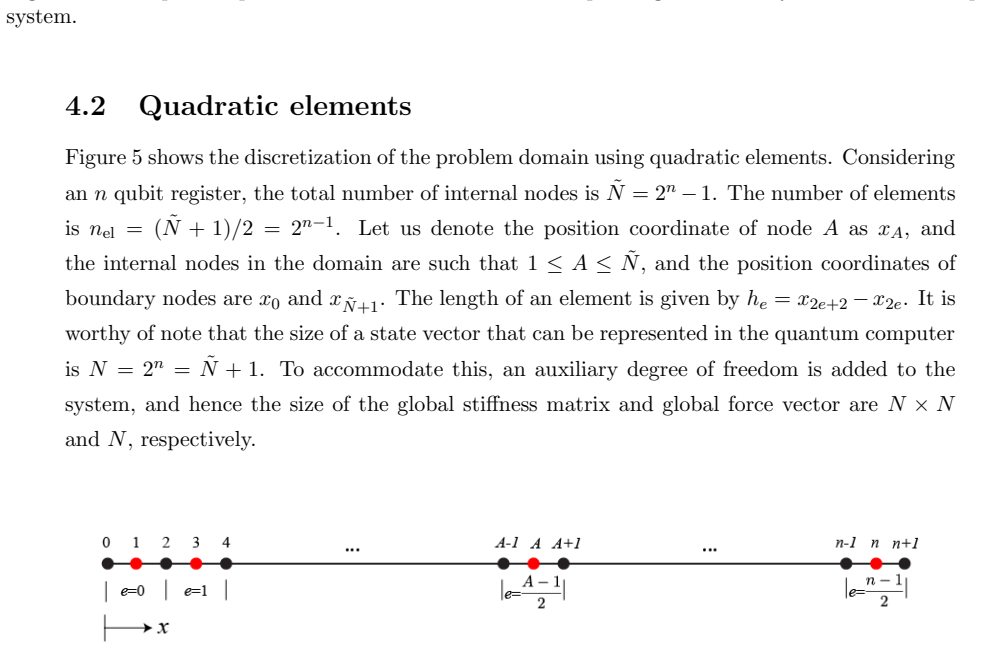
The load-bearing object is the generator function $G(e,m)$ together with the direct-stiffness assembly $K = \sum_e K^e$. Each global element matrix $K^e$ is written as a linear combination of unitaries, and the generator function selects the corresponding circuit from a small library of controlled Pauli, swap, and rotation circuits indexed by element position. Concatenation of identical non-interacting elements reduces the unitary count to 4 for a completely homogeneous linear discretization and to 8 plus one auxiliary unitary for quadratic elements. These unitaries enter the VQLS cost function through Hadamard tests, with the angle parameters supplied by a hardware-efficient ansatz of $R_y$ rotations and entangling gates.
What would settle it
Directly multiply out the right-hand side of Eq. (19) for a four-qubit linear-element discretization with nonuniform element lengths and coefficients; if the resulting matrix differs from the FEM global stiffness matrix, the unitary decomposition at the heart of Q-FEM is wrong. This is a purely classical calculation and settles the central construction claim.
Extended reading notes
Core claim
The paper's primary claim is that the finite element construction procedure can be used to obtain a unitary representation of the global stiffness matrix, and that this representation gives an efficiency advantage over generic matrix decomposition algorithms. In Q-FEM, the global stiffness matrix is assembled from global element stiffness matrices, each expressed as a sum of a small number of unitaries: two per linear element and four per quadratic element. Explicit generator functions map each unitary to a quantum circuit built from controlled Pauli-X gates, swap gates, and controlled rotations, so the decomposition is ready for execution rather than requiring numerical discovery of Pauli coefficients. As a result, heterogeneous discretizations with different element lengths and material coefficients remain fully supported, and the stiffness matrix decomposition uses O(N) unitaries in the fully heterogeneous case and a constant number in the homogeneous case.
Load-bearing premise
The load-bearing premise is that the chosen variational ansatz can represent the solution with a manageable number of parameters and that the classical optimizer can actually find the global minimum of the VQLS cost function; the paper itself shows this breaks down beyond four qubits without a classical FEM initial guess.
Editorial extensions
If this is right
- Any one-dimensional FEM stiffness matrix can be handed to VQLS as a short list of unitaries with explicit circuits, bypassing the expensive generic Pauli decomposition.
- Variable element lengths and material coefficients do not break the circuit construction, so heterogeneous meshes are handled at no extra conceptual cost.
- The same unitary library can be reused by other quantum linear solvers, not only VQLS, since the output is an explicit circuit-level representation of the stiffness matrix.
- Scaling tests indicate that FEM stiffness matrices have condition numbers growing like $N^2$, so larger problems need preconditioning or better ansatzes to avoid barren plateaus.
- For homogeneous problems the unitary count is constant but circuit depth grows with $N$, which limits near-term hardware before fault tolerance arrives.
Reading between the lines
- The measured parameter growth is exponential in qubit number but only linear in matrix size; whether this erases the hoped-for quantum advantage depends on comparing total classical-equivalent cost, which the paper does not do.
- A natural extension would be to apply the generator-function idea to two- and three-dimensional element matrices by expressing each element block as a tensor product of one-dimensional unitaries; the paper notes the extension is non-trivial but does not attempt it.
- The reliance on classical FEM initial guesses beyond four qubits suggests a testable benchmark: count the total classical work including initialization and compare it with a classical FEM solve to see where the crossover lies.
- Preconditioned stiffness matrices would be a concrete next experiment: if conditioning is reduced to near-constant, the paper's own analysis predicts fewer barren-plateau failures, which can be checked directly.
Editorial analysis
A structured set of objections, weighed in public.
Referee Report
Summary. The manuscript proposes Q-FEM, a variational quantum linear solver (VQLS) framework for finite element problems. The central construction is a unitary decomposition of the global stiffness matrix obtained by applying the direct stiffness assembly procedure: each element matrix is expressed as a linear combination of identity, permutation (X-type), and controlled phase (I^-1, Z) unitaries, and generator functions map element indices to explicit quantum circuits. Concatenation of identical non-interacting elements reduces the number of unitaries for structured grids. The method is applied to the one-dimensional steady-state heat equation with linear and quadratic elements, variable element lengths, variable coefficients, and several boundary conditions, with verification on the IBM Qiskit Aer simulator. The paper claims a significant efficiency advantage over generic matrix decomposition algorithms and gives a heuristic complexity estimate, while also reporting that the number of variational ansatz parameters grows with system size and that conditioning leads to barren-plateau-like convergence difficulties.
Significance. The unitary-construction contribution is coherent and potentially useful: it provides explicit circuits for the exact decomposition of FEM element matrices, and the numerical tests show that the constructed circuits reproduce classical FEM results for the small systems considered. The condition-number scaling matches the known theoretical bound. However, the paper's central efficiency and scalability claims are not supported by the evidence it presents. The complexity analysis in Section 4.4 omits the ansatz parameter count and circuit depth from the total resource count, and Table 3 shows that the required ansatz parameter count grows roughly exponentially with qubit number. In addition, the scaling verification for n >= 5 is warm-started from the classical FEM solution, making the reported agreement with the classical solution partially circular. The significance of the work is therefore conditional: the decomposition algebra is a genuine contribution, but the claimed advantage over generic decompositions and the exponential-advantage speculation require substantial revision or removal.
major comments (3)
- [Section 4.4 and Table 3] The claim that Q-FEM has exponential advantage when L^2 = O(1) is not supported by the paper's own data. The complexity expression O(L^2 P kappa log(1/epsilon) (log N)^m) uses P ambiguously: in Eq. (10) P denotes the number of ansatz parameters, while in Section 4.4 P is defined as the number of shots. Even under the authors' reading, the expression omits the ansatz parameter count and the transpiled circuit depth, both of which are part of the total VQLS cost. Table 3 reports ansatz parameter counts 9, 20, 42, 84, and 161 for n = 3,...,7, i.e., roughly 2^n, and Table 4 reports transpiled circuit depths up to 265,594 at n = 7. Consequently, keeping L constant does not yield a subexponential total cost, and the conclusion that Q-FEM has exponential advantage over classical FEM does not follow. The Section 1 statement of a 'significant efficiency advantage' should be revised or substantiated with a complete resource count that includes ansatz parameters, circuit depth, and shot complexity.
- [Section 5.3] The numerical scaling demonstration is partly circular. The text states: 'To solve problems with more than 4 qubits, we use the classical FEM solution to obtain a good initial guess for the parameters in the ansatz.' The results in Figure 16 then compare the Q-FEM solution with the classical FEM solution. Agreement under this protocol is not independent evidence that the variational optimization scales to larger problem sizes; it shows that the circuit construction plus local optimization around a classically obtained solution can reproduce that solution. The claim that Q-FEM converges to the correct solution for increasing problem sizes should be qualified accordingly. In addition, the manuscript does not describe how the classical FEM solution is converted into ansatz parameters, which is needed to assess the cost and possible classical overhead of the initialization step.
- [Table 1, Section 4.3] The efficiency comparison in Table 1 is incomplete. It compares only the number of unitaries in the matrix decomposition, but the total quantum cost is determined by circuit depth and gate counts as well. For the completely homogeneous case the proposed method uses only 4 unitaries, yet Section 4.3 and Figure 9 show that the concatenated circuit depth grows as O(N), and Table 4 reports steep growth of transpiled circuit depth and gate counts with qubit number. Therefore, the unitary-count reduction does not by itself establish an efficiency advantage over the decomposition in Ref. [52]. The comparison should be extended to include circuit depth, two-qubit gate counts, and the ansatz and shot contributions to the overall VQLS complexity.
minor comments (5)
- [Abstract] The sentence 'the number of parameters for the variational ansatz scale exponentially with the number of qubits, and increases the odds of convergence' is grammatically incomplete and logically unclear; please clarify whether the exponential parameter growth increases the probability of finding a solution in the tested cases.
- [Section 4.4] The symbol P denotes both the number of ansatz parameters (Eq. (10)) and the number of shots in the complexity expression of Section 4.4. Use distinct notation, for example P_theta and S, to avoid confusion.
- [Table 1] The table's column layout is confusing: it appears to compare 'Linear (Proposed)', 'Linear [52]', and 'Quadratic (Proposed)', but no quadratic decomposition from Ref. [52] is listed. A footnote explaining that the homogeneous case trades unitary count for O(N) circuit depth would help readers interpret the comparison.
- [Figures 10 and 11] The text states that various circuit characteristics 'asymptote' to O(n^3.1), O(n^4), O(n^7.5), etc., but the data cover only n = 3,...,7. These are empirical fits, not asymptotic scalings, and should be described as such.
- [Section 5.3] The convergence tolerance for the scaling study is Cp <= 2.5 x 10^-3, which is substantially looser than the tolerances used in earlier sections (for example, 10^-6 in Section 5.1 and 0.5 x 10^-5 in Section 5.2). Please state whether the reported agreement in Figure 16 is sensitive to this looser tolerance.
Circularity Check
Scaling validation is warm-started from the classical FEM solution, making the n≥5 agreement partly circular; the exact unitary decomposition itself is self-contained.
-
fitted input called prediction
[Section 5.3, 'Problem scaling' (around Fig. 16 and Table 3)]
"To solve problems with more than 4 qubits, we use the classical FEM solution to obtain a good initial guess for the parameters in the ansatz. ... Using the generated initial guesses for parameters in the ansatz, we obtain solutions with the Q-FEM framework for increasing problem sizes, which are in good agreement with the classical solution, as shown in Fig. 16."
For n≥5, the quantity being verified (agreement with the classical FEM solution) is used to construct the optimizer's starting point: classical FEM amplitudes are converted into ansatz parameters. The subsequent agreement is therefore not an independent prediction of the solver; it is a warm-started confirmation biased toward the reference solution. In addition, Table 3's layer depths are chosen per problem size 'to obtain a correct solution', so the reported exponential parameter growth is a fitted requirement rather than a predicted scaling law. This makes the large-system convergence evidence circular, while leaving the exactness of the unitary decomposition itself unaffected.
full rationale
The core derivation in Sections 3–4 is not circular. Equations (19) and (27) give exact linear-combination-of-unitaries representations of the assembled FEM stiffness matrix, and Sections 4.1.1 and 4.2.1 construct explicit circuits for each unitary via generator functions; no fitted parameter enters the decomposition and no self-citation supplies a load-bearing premise. The numerical verification at n=3 and n=4 uses random initial parameters and is independent. The only circular step is the large-scale validation: for n≥5 the ansatz is initialized from the classical FEM solution and then reported to agree with the classical FEM solution, so that agreement is partly forced by construction. The Section 4.4 exponential-advantage claim also omits the ansatz parameter count and transpiled circuit depth (Tables 3 and 4), but that is an unsupported complexity inference rather than a circular reduction, so it is not scored here. Overall, the central unitary-construction contribution is self-contained; the circularity is confined to the scaling validation, which warrants a moderate score.
Assumptions & free parameters
free parameters (3)
- Ansatz layer depth per qubit count =
n=3:2, n=4:4, n=5:6, n=6:13, n=7:22 (Table 3)
- Penalty parameter P =
100
- Convergence tolerance for cost function =
1e-6, 5e-6, 2.5e-3, 1e-3 across experiments
assumptions (4)
- standard math The VQLS cost function minimum corresponds to the solution of the linear system (Section 2.2, Eq. 8)
- standard math The Mottonen state preparation circuit loads the force vector with depth O(N) and the stated rotation angles (Section 2.1)
- ad hoc to paper The chosen hardware-efficient ansatz can represent the FEM solution (Sections 5.1, 5.3)
- domain assumption Qiskit Aer noiseless simulation faithfully represents ideal quantum circuit behavior (Section 5)
Cite this review
Pith. "Pith review of An Implementation of the Finite Element Method in Hybrid Classical/Quantum Computers." pith.science (2026). https://pith.science/paper/KILECTTK
@misc{pith2026241109038,
  author       = {Pith},
  title        = {Pith review of: An Implementation of the Finite Element Method in Hybrid Classical/Quantum Computers},
  year         = {2026},
  howpublished = {\url{https://pith.science/paper/KILECTTK}},
  note         = {Machine review of arXiv:2411.09038}
}
read the original abstract
This manuscript presents the Quantum Finite Element Method (Q-FEM) developed for use in noisy intermediate-scale quantum (NISQ) computers and employs the variational quantum linear solver (VQLS) algorithm. The proposed method leverages the classical FEM procedure to perform the unitary decomposition of the stiffness matrix and employs generator functions to design explicit quantum circuits corresponding to the unitaries. Q-FEM keeps the structure of the finite element discretization intact allowing for the use of variable element lengths and material coefficients in FEM discretization. The proposed method is tested on a steady-state heat equation discretized using linear and quadratic shape functions. Numerical verification studies are performed on the IBM QISKIT simulator and it is demonstrated that Q-FEM is effective in converging to the correct solution for a variety of problems and model discretizations, including with different element lengths, variable coefficients, and different boundary conditions. The formalism developed herein is general and can be extended to problems with higher dimensions. However, numerical examples also demonstrate that the number of parameters for the variational ansatz scale exponentially with the number of qubits, and increases the odds of convergence. Moreover, the deterioration of system conditioning with problem size results in barren plateaus and convergence difficulties.
Figures


Figures from the paper (16 more)



Reference graph
Works this paper leans on
-
[52]
C. J. Trahan, M. Loveland, N. Davis, and E. Ellison. A variational quantum linear solver application to discrete finite-element methods. Entropy, 25(4):580, 2023
work page 2023
- [1]
-
[2]
M. Ali and M. Kabel. Performance study of variational quantum algorithms for solving the poisson equation on a quantum computer. Phys. Rev. Appl. , 20:014054, Jul 2023. doi: 10.1103/PhysRevApplied.20.014054. URL https://link.aps.org/doi/10.1103/ PhysRevApplied.20.014054
- [3]
-
[4]
I. F. Araujo, D. K. Park, F. Petruccione, and A. J. da Silva. A divide-and-conquer algorithm for quantum state preparation. Scientific Reports , 11(1):6329, March 2021. ISSN 2045-2322. doi: 10.1038/s41598-021-85474-1. URL https://doi.org/10.1038/ s41598-021-85474-1
-
[5]
J. Bausch. Fast Black-Box Quantum State Preparation. Quantum, 6:773, August 2022. ISSN 2521-327X. doi: 10.22331/q-2022-08-04-773. URL https://doi.org/10.22331/ q-2022-08-04-773
-
[6]
P. Bermejo, B. Aizpurua, and R. Or´ us. Improving gradient methods via coordinate transformations: Applications to quantum machine learning. Phys. Rev. Res. , 6:023069, Apr 2024. doi: 10.1103/PhysRevResearch.6.023069. URL https://link.aps.org/doi/ 10.1103/PhysRevResearch.6.023069
-
[7]
C. Bravo-Prieto, R. LaRose, M. Cerezo, Y. Subasi, L. Cincio, and P. J. Coles. Variational quantum linear solver. Quantum, 7:1188, 2023
work page 2023
Show all 58 references
-
[8]
G. K. Brennen. An observable measure of entanglement for pure states of multi-qubit systems. Quantum Info. Comput. , 3(6):619–626, November 2003. ISSN 1533-7146. 41
2003
-
[9]
Y. Cao, A. Papageorgiou, I. Petras, J. Traub, and S. Kais. Quantum algorithm and circuit design solving the poisson equation. New Journal of Physics , 15(1):013021, 2013
2013
-
[11]
Cerezo, A
M. Cerezo, A. Sone, T. Volkoff, L. Cincio, and P. J. Coles. Cost function dependent barren plateaus in shallow parametrized quantum circuits. Nature Communications, 12 (1):1791, March 2021. ISSN 2041-1723. doi: 10.1038/s41467-021-21728-w. URL https: //doi.org/10.1038/s41467-02...
2021 doi
-
[12]
Chakraborty, A
S. Chakraborty, A. Gily´ en, and S. Jeffery. The power of block-encoded matrix pow- ers: improved regression techniques via faster hamiltonian simulation. arXiv preprint arXiv:1804.01973, 2018
2018 arXiv
-
[13]
A. M. Childs, R. Kothari, and R. D. Somma. Quantum algorithm for systems of lin- ear equations with exponentially improved dependence on precision. SIAM Journal on Computing, 46(6):1920–1950, 2017
1920
-
[14]
B. D. Clader, B. C. Jacobs, and C. R. Sprouse. Preconditioned quantum linear system algorithm. Physical review letters , 110(25):250504, 2013
2013
-
[15]
Cleve, A
R. Cleve, A. Ekert, C. Macchiavello, and M. Mosca. Quantum algorithms revisited. Pro- ceedings of the Royal Society of London. Series A: Mathematical, Physical and Engineering Sciences, 454(1969):339–354, 1998
1969
-
[16]
F. M. Creevey, C. D. Hill, and L. C. L. Hollenberg. GASP: a genetic algorithm for state preparation on quantum computers. Scientific Reports , 13(1):11956, July 2023. ISSN 2045-2322. doi: 10.1038/s41598-023-37767-w. URL https://doi.org/10.1038/ s41598-023-37767-w
2023 doi
-
[17]
Fa ´ ılde, J
D. Fa ´ ılde, J. D. Viqueira, M. Mussa Juane, and A. G´ omez. Using differential evolution to avoid local minima in variational quantum algorithms. Scientific Reports, 13(1):16230, 2023
2023
-
[18]
Feniou, O
C. Feniou, O. Adjoua, B. Claudon, J. Zylberman, E. Giner, and J.-P. Piquemal. Sparse quantum state preparation for strongly correlated systems. The Journal of Physical Chemistry Letters , 15(11):3197–3205, 2024. doi: 10.1021/acs.jpclett.3c03159. URL https://doi.org/10.1021/acs...
2024 doi
-
[19]
B. T. Gard, L. Zhu, G. S. Barron, N. J. Mayhall, S. E. Economou, and E. Barnes. Efficient symmetry-preserving state preparation circuits for the variational quantum eigensolver algorithm. npj Quantum Information , 6(1):10, January 2020. ISSN 2056-6387. doi: 10.1038/s41534-019-...
2020 doi
-
[20]
A. W. Harrow and J. C. Napp. Low-depth gradient measurements can improve conver- gence in variational hybrid quantum-classical algorithms. Phys. Rev. Lett. , 126:140502, Apr 2021. doi: 10.1103/PhysRevLett.126.140502. URL https://link.aps.org/doi/ 10.1103/PhysRevLett.126.140502
2021 doi
-
[21]
A. W. Harrow, A. Hassidim, and S. Lloyd. Quantum algorithm for linear systems of equations. Physical review letters , 103(15):150502, 2009
2009
-
[22]
˙Zyczkowski and H-J
K. ˙Zyczkowski and H-J. Sommers. Average fidelity between random quantum states. Phys. Rev. A , 71:032313, Mar 2005. doi: 10.1103/PhysRevA.71.032313. URL https: //link.aps.org/doi/10.1103/PhysRevA.71.032313
2005 doi
-
[23]
R. Iten, R. Colbeck, I. Kukuljan, J. Home, and M. Christandl. Quantum circuits for isometries. Phys. Rev. A , 93:032318, Mar 2016. doi: 10.1103/PhysRevA.93.032318. URL https://link.aps.org/doi/10.1103/PhysRevA.93.032318
2016 doi
-
[24]
Khatri, R
S. Khatri, R. LaRose, A. Poremba, L. Cincio, A. T. Sornborger, and P. J. Coles. Quantum- assisted quantum compiling. Quantum, 3:140, 2019
2019
-
[25]
M. Kus, J. Mostowski, and F. Haake. Universality of eigenvector statistics of kicked tops of different symmetries. Journal of Physics A: Mathematical and General , 21(22): L1073, 1988. doi: 10.1088/0305-4470/21/22/006. URL https://dx.doi.org/10.1088/ 0305-4470/21/22/006
1988 doi
-
[26]
LaRose, A
R. LaRose, A. Tikku, ´E. O’Neel-Judy, L. Cincio, and P. J. Coles. Variational quantum state diagonalization. npj Quantum Information , 5(1):57, 2019
2019
-
[27]
J. Lee, A. B. Magann, H. A. Rabitz, and C. Arenz. Progress toward favorable land- scapes in quantum combinatorial optimization. Phys. Rev. A , 104:032401, Sep 2021. doi: 10.1103/PhysRevA.104.032401. URL https://link.aps.org/doi/10.1103/PhysRevA. 104.032401
2021 doi
-
[28]
Leone, S
L. Leone, S. F. E. Oliviero, L. Cincio, and M. Cerezo. On the practical usefulness of the hardware efficient ansatz. Quantum, 8:1395, 2024
2024
-
[29]
S. Levy. Structural analysis and influence coefficients for delta wings. Journal of the Aeronautical Sciences, 20(7):449–454, 1953. 43
1953
-
[30]
Liu, Y.-S
H.-L. Liu, Y.-S. Wu, L.-C. Wan, S.-J. Pan, S.-J. Qin, F. Gao, and Q.-Y. Wen. Variational quantum algorithm for the poisson equation. Physical Review A , 104(2):022418, 2021
2021
-
[31]
Y. Liu, J. Liu, J. R. Raney, and P. Wang. Quantum computing for solid mechanics and structural engineering–a demonstration with variational quantum eigensolver. Extreme Mechanics Letters, 67:102117, 2024
2024
-
[32]
D. Lu, Z. Wang, J. Liu, Y. Li, W.-B. Ewe, and Z. Liu. From ad-hoc to systematic: A strategy for imposing general boundary conditions in discretized pdes in variational quantum algorithm. arXiv preprint arXiv:2310.11764 , 2023
-
[33]
O. R. Meitei, B. T. Gard, G. S. Barron, D. P. Pappas, S. E. Economou, E. Barnes, and N. J. Mayhall. Gate-free state preparation for fast variational quantum eigensolver simulations. npj Quantum Information , 7(1):155, October 2021. ISSN 2056-6387. doi: 10.1038/s41534-021-00493...
2021 doi
-
[34]
D. A. Meyer and N. R. Wallach. Global entanglement in multiparticle systems. Journal of Mathematical Physics , 43(9):4273–4278, September 2002. ISSN 0022-
2002
-
[35]
Montanaro and S
A. Montanaro and S. Pallister. Quantum algorithms and the finite element method. Physical Review A , 93(3):032324, 2016
2016
-
[36]
Mottonen, J
M. Mottonen, J. J. Vartiainen, V. Bergholm, and M. M. Salomaa. Transformation of quantum states using uniformly controlled rotations. arXiv preprint quant-ph/0407010 , 2004
2004 arXiv
-
[37]
Nguyen, L
V.-D. Nguyen, L. Wu, F. Remacle, and L. Noels. A quantum annealing-sequential quadratic programming assisted finite element simulation for non-linear and history- dependent mechanical problems. European Journal of Mechanics - A/Solids , 105:105254,
-
[38]
M. R. Perelshtein, A. I. Pakhomchik, A. A. Melnikov, A. A. Novikov, A. Glatz, G. S. Paraoanu, V. M. Vinokur, and G. B. Lesovik. Solving large-scale linear systems of equa- tions by a quantum hybrid algorithm. Annalen der Physik , 534(7), May 2022. ISSN 1521-3889. doi: 10.1002/...
2022 doi
-
[39]
R. M. N. Pesce and P. D. Stevenson. H2zixy: Pauli spin matrix decomposition of real symmetric matrices. arXiv preprint arXiv:2111.00627 , 2021
2021 arXiv
-
[40]
Plesch and C
M. Plesch and C. Brukner. Quantum-state preparation with universal gate decompo- sitions. Phys. Rev. A , 83:032302, Mar 2011. doi: 10.1103/PhysRevA.83.032302. URL https://link.aps.org/doi/10.1103/PhysRevA.83.032302
2011 doi
-
[41]
Preskill
J. Preskill. Quantum computing in the nisq era and beyond. Quantum, 2:79, 2018
2018
-
[42]
O. M. Raisuddin and S. De. Feqa: Finite element computations on quantum annealers. Comput. Methods. Appl. Mech. Engrg. , 395:115014, 2022
2022
-
[43]
O. M. Raisuddin and S. De. Quantum relaxation for linear systems in finite element analysis, 2023. URL https://arxiv.org/abs/2308.01377
2023 arXiv
-
[44]
O. M. Raisuddin and S. De. Quantum multigrid algorithm for finite element problems. arXiv preprint arXiv:2404.07466 , 2024
2024 arXiv
-
[45]
Renaud, P
N. Renaud, P. Rodr ´ ıguez-S´ anchez, J. Hidding, and P. C. Broekema. Quantum radio astronomy: Quantum linear solvers for redundant baseline calibration. Astronomy and Computing, page 100803, 2024
2024
-
[46]
V. V. Shende, S. S. Bullock, and I. L. Markov. Synthesis of quantum-logic circuits. IEEE Transactions on Computer-Aided Design of Integrated Circuits and Systems , 25(6): 1000–1010, 2006. doi: 10.1109/TCAD.2005.855930
2006
-
[47]
S. Sim, P. D. Johnson, and A. Aspuru-Guzik. Expressibility and entangling capability of parameterized quantum circuits for hybrid quantum-classical algorithms.Advanced Quan- tum Technologies, 2(12), October 2019. ISSN 2511-9044. doi: 10.1002/qute.201900070. URL http://dx.doi.o...
2019 doi
-
[48]
Srivastava and V
S. Srivastava and V. Sundararaghavan. Box algorithm for the solution of differential equations on a quantum annealer. Physical Review A , 99(5), May 2019. ISSN 2469-
2019
-
[49]
Strang and G
G. Strang and G. Fix. An Analysis of the Finite Element Methods, 2nd Edition and Engineering. Wellesley-Cambridge Press, Philadelphia, PA, 2008. doi: 10.1137/1. 9780980232707. URL https://epubs.siam.org/doi/abs/10.1137/1.9780980232707. 45
2008 doi
-
[50]
Suba¸ sı, R
Y. Suba¸ sı, R. D. Somma, and D. Orsucci. Quantum algorithms for systems of linear equa- tions inspired by adiabatic quantum computing. Physical review letters , 122(6):060504, 2019
2019
-
[51]
Tilly, H
J. Tilly, H. Chen, S. Cao, D. Picozzi, K. Setia, Y. Li, E. Grant, L. Wossnig, I. Rungger, G. H. Booth, and J. Tennyson. The variational quantum eigensolver: A review of methods and best practices. Physics Reports, 986:1–128, 2022. ISSN 0370-1573. doi: https://doi. org/10.1016/...
2022 doi
-
[53]
Wossnig, Z
L. Wossnig, Z. Zhao, and A. Prakash. Quantum linear system algorithm for dense matri- ces. Physical review letters , 120(5):050502, 2018
2018
-
[54]
Zhang, C
H.-K. Zhang, C. Zhu, G. Liu, and X. Wang. Fundamental limitations on optimization in variational quantum algorithms. arXiv preprint arXiv:2205.05056 , 2022
2022 arXiv
-
[55]
Zhou and S
Z. Zhou and S. Keller. Improving convergence by optimizing the condition number of the stiffness matrices arising from least-squares finite element methods. Computer Methods in Applied Mechanics and Engineering , 385:114023, 2021
2021
-
[56]
Zlokapa, B
A. Zlokapa, B. Villalonga, S. Boixo, and D. A. Lidar. Boundaries of quantum supremacy via random circuit sampling. npj Quantum Information , 9(1):36, 2023. 46
2023
-
[2024]
doi: https://doi.org/10.1016/j.euromechsol.2024.105254
ISSN 0997-7538. doi: https://doi.org/10.1016/j.euromechsol.2024.105254. URL https://www.sciencedirect.com/science/article/pii/S0997753824000342
2024
-
[2488]
URL https://doi.org/10.1063/1.1497700
doi: 10.1063/1.1497700. URL https://doi.org/10.1063/1.1497700. eprint: https://pubs.aip.org/aip/jmp/article-pdf/43/9/4273/19183190/4273 1 online.pdf
-
[9934]
URL http://dx.doi.org/10.1103/PhysRevA
doi: 10.1103/physreva.99.052355. URL http://dx.doi.org/10.1103/PhysRevA. 99.052355
Reviewed August 12, 2026 · model on record in the stance chip above.
Discussion (0). Continue with ORCID to comment.