REVIEW 5 major objections 5 minor 61 references
Early Detection of Multiwavelength Blazar Variability
T0 review · 5 major / 5 minor · reviewed 2026-08-12 · deepseek-v4-flash
Pith's one-line read An unsupervised deep-learning pipeline detects flaring states in multiwavelength blazar light curves without needing labeled flare examples.
desk verdict A useful, well-documented anomaly-detection framework with public code, but the headline claim of reliable historical detection is weakened by an in-sample evaluation that removes the ground-truth flares from the training background. read the letter →
The pith
A machine-rendered reading of the paper's core claim, the machinery that carries it, and where it could break.
The reading
What carries the argument
The core mechanism is an encoder-decoder recurrent neural network that forecasts background activity from a context window, followed by a variational autoencoder that maps the residuals (data minus forecast) into an embedding vector. A Bayesian Gaussian mixture model then scores how far an embedding lies from background, while the autoencoder's reconstruction error catches out-of-distribution states; the two p-values are combined into a single significance. Temporal weights suppress old anomalies in sparse channels, and uncertainty resampling propagates measurement errors into the final significance.
What would settle it
Take the BL Lacertae light curves, intentionally leave a weak flare (below the γsignoise = 5 cutoff) in the training data, retrain the pipeline, and check whether the calibrated significance for known historical flares decreases; a shift would show the background model is contaminated.
Extended reading notes
Core claim
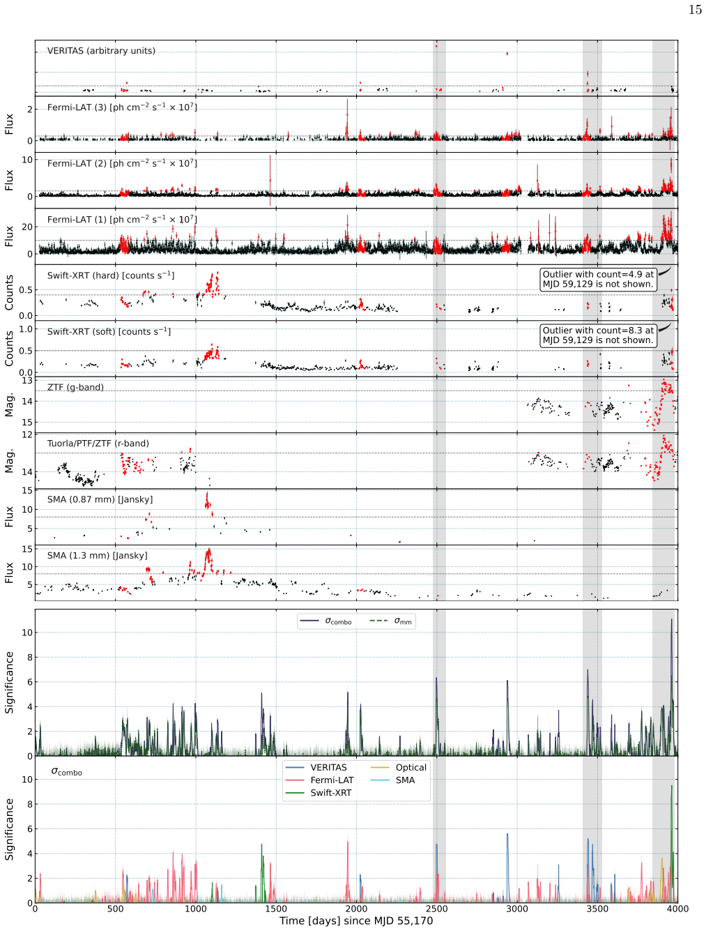
The central claim is that an unsupervised anomaly-detection pipeline, trained only on cleaned background activity, can reliably flag flaring states in real-world multiwavelength light curves and can hint at precursors before the flare fully develops. On eleven years of BL Lacertae data spanning very-high-energy gamma rays to radio, the framework recovers five known VHE flares at multi-sigma significance, and in the 2019–2020 episodes it reached 3σ on the optical and gamma-ray precursor two to four days before the community's alerts. The detection is carried by two complementary test statistics: a mixture-model compatibility in a learned embedding space and a reconstruction-error statistic that catches states too novel for the embedding to represent.
Load-bearing premise
The framework defines 'anomaly' relative to a training sample that is assumed to be pure background, but that sample is produced by manually removing flaring intervals and applying per-channel variability cutoffs, so any hidden flares left in the background or any normal variability removed will bias the anomaly scores.
Editorial extensions
If this is right
- The pipeline yields a single, calibrated significance per time step across all channels, so observatories can trigger VHE follow-up on a common numeric threshold.
- Historical BL Lacertae analysis shows detections at the same time or earlier than the community's alert system, including a 3σ precursor before the 2020 optical and gamma-ray maximum.
- The framework detects downward anomalies and cross-channel correlations, not just elevated fluxes, expanding the kinds of flaring states that can trigger alerts.
- Measurement uncertainties propagate to the significance, so a low-quality outlier carries a large uncertainty and can be recognized as a likely false positive.
- The method is built for real-time use and can be deployed in an automated alert broker without labeled flare data.
Reading between the lines
- If the background model generalizes, the same pipeline could be applied to other blazars or to transients like tidal disruption events, wherever a quiescent baseline can be defined.
- The authors leave timescale flexibility implicit: an ensemble of pipelines with different time-bin widths could cover hour-to-week variability and might reveal precursors that day-binned analysis misses.
- A direct test suggested by the approach is to run the framework on a second well-monitored blazar with known historical flares and compare detection times against the published alert record.
- The definition of anomaly depends on the cleaned training sample, so the method's 'anomaly' is source-specific rather than universal; transferring it to a new source would require retraining on that source's own quiescent states.
Signed reviews
Editorial analysis
A structured set of objections, weighed in public.
Referee Report
Summary. The paper presents a deep-learning anomaly-detection framework for multiwavelength blazar light curves. The pipeline uses an RNN forecaster to predict background activity, an autoencoder to embed weighted residuals, and a Bayesian Gaussian mixture model to characterize background states; two test statistics (reconstruction error and mixture-model compatibility) are combined into a calibrated significance. The method is evaluated on simulations of the blazar 1ES 1215+303 in Fermi-LAT and CTAO bands and on historical multiwavelength data of BL Lacertae (VERITAS, Fermi-LAT, Swift-XRT, optical, SMA). The authors report that the framework detects known historical flares, sometimes earlier than the community alerts, and can hint at precursors.
Significance. If the central validation were out-of-sample, the framework would be a useful real-time tool for triggering IACT observations and for standardizing multiwavelength flare alerts. The paper has clear strengths: the code and simulation data are publicly available, measurement uncertainties are propagated through the pipeline, the simulations use realistic instrument responses, and the architecture is described in enough detail to be reproduced. However, the headline claim is currently supported only by an in-sample evaluation, so the significance of the result is conditional on a successful out-of-sample test.
major comments (5)
- [§4.1, §4.3, §4.4] The historical evaluation is in-sample with respect to the definition of ground truth. In §4.1 the training background is constructed by manually removing the VERITAS flaring intervals at MJDs 55,725, 57,200, 57,675, 58,100, 58,600 (plus 50-day buffers and per-channel cutoffs), and the high-significance peaks reported in §4.3 (t=2,500, 2,900, 3,400) and in Table 2 coincide with those same excluded intervals. A detector trained on the complement of the rule that flags those intervals will tend to flag them, so the reported detections and precursors may encode the cleaning thresholds rather than a learned multiwavelength precursor pattern. Please add a temporal out-of-sample test (e.g., train only on data before a cut date and evaluate after, or leave-one-flare-out) and report the false-alarm rate on quiescent periods; without such a control the headline claim in §4.4 is not established.
- [§3.4, §3.6] The simulation study is not an independent blind test. The light curves are generated from the 2017 steady-state spectrum of 1ES 1215+303, and the injected flares are scaled versions of the same Fref template (Valverde et al. 2020) used to define the source; the background is simulated from the same spectral model rather than cleaned real data. The observed scaling of significance with flare strength and coverage (Fig. 5) is a useful sensitivity check, but it cannot calibrate the historical comparison because there is no unknown signal and no realistic correlated multiwavelength background. Please either add a validation on a second source or on a held-out flare template/epoch, or explicitly restrict the simulation to a sensitivity study and base the detection claim solely on an out-of-sample real-data test.
- [Eq. (1)] Equation (1) is internally inconsistent with the intended behavior of the temporal weights. For tstep - tdelay > 1, the factor (1 - max(0, tstep - tdelay)) is negative; with gamma_decay = 1 this gives a negative weight, and with non-integer gamma_decay it gives a complex value, whereas the text and Fig. 2 describe weights that decay from unity toward zero. If this is a typo, please correct the sign (e.g., (1 + max(0, tstep - tdelay))^{-gamma_decay}) and confirm that the implementation matches; if the formula is correct, please explain how negative/complex weights are handled, since this equation controls the entire embedding input in §2.3.
- [§3.1, §3.2] The cleaning and augmentation procedure trains the background on data whose temporal ordering and inter-band correlations have been deliberately destroyed: data are shuffled inside each window, timestamps are randomized, and independent global shifts are applied per channel. The paper motivates the framework by sensitivity to 'subtle correlations across bands' (§1) and reports precursor signals that are inter-channel (§4.3.3), but no validation is shown that the correlation-free null distribution used for calibration matches real quiescent BL Lac activity. If real quiescent data contain residual correlations, the significance calibration will be systematically liberal. Please quantify this by comparing the background model distribution to un-cleaned quiescent data, or by demonstrating on simulations with correlated background that the false-alarm rate is controlled.
- [§4.3.3, Table 2] The 'same time or earlier than the state-of-the-art' claim is not supported by a defined detection threshold. Several entries in Table 2 are called detections or precursors at 1.3–2.5σ (e.g., t=3,434–3,435, t=570, t=3,940), while others are quoted at 3–10σ; the paper never states the significance threshold used to decide that an event was 'detected' by the framework, nor the expected number of false alarms over the 4,000-day baseline. Please specify the decision rule, compute the false-alarm rate from the null distribution, and report the resulting detection time for each event at a fixed threshold.
minor comments (5)
- [§3.5] The sentence 'm = 10 context steps and n = 5 search steps' is inconsistent with Table 1 and §2.1, where n is the context and m is the search window; please correct the notation.
- [Abstract, §4.4] The phrase 'without the need for a labeled training data set of flaring states' is misleading because §4.1 manually labels flaring intervals for exclusion; consider rephrasing to 'without labeled flaring states in the training target' or similar.
- [Data Availability] The GitLab URL in the Data Availability section contains a space ('trans finder/blazar flares') and should be replaced with the actual URL.
- [Figure 7/8] The VERITAS panels show counts in arbitrary units modified by random noise; the text states that the pipeline uses the true flux, but the figure caption should explicitly state that the displayed counts are a proxy so that readers do not misinterpret the scaling.
- [Introduction] The Introduction refers to 'Sect. 3.3' for the simulation study, but the simulation is actually described in §3.4–§3.6; please fix the cross-reference.
Circularity Check
Historical evaluation is in-sample: the training background is defined by excising the same VERITAS flares (plus 50-day buffers) that are then reported as detections, so the headline claim is partly forced by the cleaning rule rather than by learned multiwavelength correlations.
-
fitted input called prediction
[Section 4.1 (historical training cleaning) and Section 4.3/Table 2 (historical results)]
"We decide to first manually exclude clearly identifiable high states from the light curves. In particular, we remove flaring states based on VERITAS data surrounding MJDs 55,725, 57,200, 57,675, 58,100 and 58,600. We exclude any data taken within 50 days of the respective VHE flares from all channels. ... In general, we find elevated significance during the parts of the light curve that were excluded for training."
The VHE flares reported as detections in Sections 4.3-4.4 (e.g., t=570, 2,496, 2,900, 3,400 in Table 2) are the same intervals removed when constructing the training background in Section 4.1, each with a 50-day buffer across all channels. All model components (forecaster, autoencoder, BGMM, significance calibration) are fitted on the complement of those intervals, and an anomaly is defined as incompatibility with that cleaned background. The excised intervals are therefore outliers by construction, not out-of-sample predictions. The paper's own statement that elevated significance appears 'during the parts of the light curve that were excluded for training' exposes this coupling. No temporal split, external epoch, or false-alarm budget separates the cleaning rule from the evaluation.
full rationale
The central circularity is the in-sample definition of the training background. In Section 4.1 the paper builds a 'background-only' dataset by manually removing VERITAS flaring states and all data within 50 days of those flares, across all channels, and then applies per-channel variability cutoffs. Section 4.3 then reports high-significance detections at exactly those removed intervals, and Section 4.4 uses these as evidence that the framework 'reliably detect[s] flares' and detects 'flaring states at the same time or earlier than the state-of-the-art.' Because the model and its calibration are trained on the complement of those intervals, the removed intervals are anomalous by construction; the historical detections are therefore a re-detection of the cleaning cuts rather than an independent forecast. The paper acknowledges this coupling only indirectly in the Discussion ('prior data cleaning is needed. This may introduce biases'), but no quantitative control is provided: there is no temporal out-of-sample split, no test on an epoch whose flares were not used to define the background, and no false-alarm budget for the historical comparison. The simulation study is not a valid control for this issue because its background is simulated and its injected flare templates are known, so it cannot calibrate the effect of cleaning real data. The 2020 precursor episode (optical rise detected at t ~ 3896, before the community ATels) is a genuinely more out-of-sample element and partially supports the method's utility, but it does not rescue the main validation of historical VHE flares. The significance-calibration prescription is taken from Sadeh (2020), a coauthor's prior work; this is self-citation, but it is a methodological reference rather than an unverified uniqueness claim, so it is not counted as circular in itself. Overall, the historical evaluation reduces in part to the data-cleaning rule, giving a partial circularity score of 6.
Assumptions & free parameters
free parameters (10)
- gamma_timeaggr =
1 day
- gamma_signoise =
5 (standard deviations)
- gamma_decay =
1
- Window sizes n, m =
n=10 context steps, m=5 search steps
- Manual exclusion radius around VHE flares =
50 days
- Channel cleaning cutoffs =
Not quantified (defined per channel variance)
- Autoencoder latent dimension =
Adaptive
- BGMM number of components =
Adaptive via MCMC
- RNN and training hyperparameters =
learning rate 0.005, dropout 10%, L2 0.0001; doubled for real data
- Augmentation amplitude ranges =
2 to 100 upward, -2 to -10 downward, duration 1 to 8 days
assumptions (5)
- domain assumption The cleaned training windows represent pure background source activity.
- domain assumption The encoder context windows are free of potential signals during forecasting.
- domain assumption The RNN provides unbiased probabilistic forecasts of background activity.
- domain assumption Measurement uncertainties are Gaussian, independent, and can be propagated by resampling.
- domain assumption The null-hypothesis distribution derived from background samples remains valid across the full search grid without explicit trial correction.
Cite this review
Pith. "Pith review of Early Detection of Multiwavelength Blazar Variability." pith.science (2026). https://pith.science/paper/JYCLYEE7
@misc{pith2026241110140,
  author       = {Pith},
  title        = {Pith review of: Early Detection of Multiwavelength Blazar Variability},
  year         = {2026},
  howpublished = {\url{https://pith.science/paper/JYCLYEE7}},
  note         = {Machine review of arXiv:2411.10140}
}
read the original abstract
Blazars are a subclass of active galactic nuclei with relativistic jets pointing toward the observer. They are notable for their flux variability at all observed wavelengths and timescales. Together with simultaneous measurements at lower energies, the very-high-energy (VHE) emission observed during blazar flares may be used to probe the population of accelerated particles. However, optimally triggering observations of blazar high states can be challenging. Notable examples include identifying a flaring episode in real time and predicting VHE flaring activity based on lower-energy observables. For this purpose, we have developed a novel deep learning analysis framework, based on data-driven anomaly detection techniques. It is capable of detecting various types of anomalies in real-world, multiwavelength light curves, ranging from clear high states to subtle correlations across bands. Based on unsupervised anomaly detection and clustering methods, we differentiate source variability from noisy background activity, without the need for a labeled training data set of flaring states. The framework incorporates measurement uncertainties and is robust given data quality challenges, such as varying cadences and observational gaps. We evaluate our approach using both historical data and simulations of blazar light curves in two energy bands, corresponding to sources observable with the Fermi Large Area Telescope and the upcoming Cherenkov Telescope Array Observatory. In a statistical analysis, we show that our framework can reliably detect known historical flares.
Figures


Figures from the paper (6 more)




Reference graph
Works this paper leans on
-
[1]
G., Ackermann, M., Adams, J., et al
Aartsen, M. G., Ackermann, M., Adams, J., et al. 2018, Science, 361, aat1378, doi: 10.1126/science.aat1378
-
[2]
Abbott, B. P., Abbott, R., Abbott, T. D., et al. 2017, Phys. Rev. Lett., 119, 161101, doi: 10.1103/PhysRevLett.119.161101
-
[3]
2022, The Astrophysical Journal Supplement Series, 260, 53, doi: 10.3847/1538-4365/ac6751
Abdollahi, S., Acero, F., Baldini, L., et al. 2022, The Astrophysical Journal Supplement Series, 260, 53, doi: 10.3847/1538-4365/ac6751
-
[4]
U., Archambault, S., Archer, A., et al
Abeysekara, A. U., Archambault, S., Archer, A., et al. 2015, The Astrophysical Journal, 815, L22, doi: 10.1088/2041-8205/815/2/l22
-
[5]
U., Benbow, W., Bird, R., et al
Abeysekara, A. U., Benbow, W., Bird, R., et al. 2018, ApJ, 856, 95, doi: 10.3847/1538-4357/aab35c
-
[6]
A., Aliu, E., Arlen, T., et al
Acciari, V. A., Aliu, E., Arlen, T., et al. 2009, The Astrophysical Journal, 693, L104, doi: 10.1088/0004-637x/693/2/l104
-
[7]
2013, Astroparticle Physics, 43, 3, doi: 10.1016/j.astropartphys.2013.01.007
Acharya, B., Actis, M., Aghajani, T., et al. 2013, Astroparticle Physics, 43, 3, doi: 10.1016/j.astropartphys.2013.01.007
-
[8]
2022, Science, 376, abn0567, doi: 10.1126/science.abn0567
Aharonian, F., Ait Benkhali, F., Ang¨ uner, E., et al. 2022, Science, 376, abn0567, doi: 10.1126/science.abn0567
Show all 61 references
-
[9]
G., Bazer-Bachi, A
Aharonian, F., Akhperjanian, A. G., Bazer-Bachi, A. R., et al. 2007, The Astrophysical Journal, 664, L71, doi: 10.1086/520635
2007 doi
-
[10]
2006, Astron
Aharonian, F., et al. 2006, Astron. Astrophys., 457, 899, doi: 10.1051/0004-6361:20065351
2006 doi
-
[11]
2008, Physics Letters B, 668, 253, doi: 10.1016/j.physletb.2008.08.053 Aleksi´ c, J., et al
Albert, J., Aliu, E., Anderhub, H., et al. 2008, Physics Letters B, 668, 253, doi: 10.1016/j.physletb.2008.08.053 Aleksi´ c, J., et al. 2016, Astroparticle Physics, 72, 76, doi: 10.1016/j.astropartphys.2015.02.005
2008 doi
-
[12]
2013, ApJ, 762, 92, doi: 10.1088/0004-637X/762/2/92
Arlen, T., Aune, T., Beilicke, M., et al. 2013, ApJ, 762, 92, doi: 10.1088/0004-637X/762/2/92
2013 doi
-
[13]
B., Abdo, A
Atwood, W. B., Abdo, A. A., Ackermann, M., et al. 2009, ApJ, 697, 1071, doi: 10.1088/0004-637X/697/2/1071
2009 doi
-
[14]
1999, A&AS, 135, 371, doi: 10.1051/aas:1999179
Ballet, J. 1999, A&AS, 135, 371, doi: 10.1051/aas:1999179
1999 doi
-
[15]
C., Kulkarni, S
Bellm, E. C., Kulkarni, S. R., Graham, M. J., et al. 2019a, PASP, 131, 018002, doi: 10.1088/1538-3873/aaecbe
-
[16]
C., Kulkarni, S
Bellm, E. C., Kulkarni, S. R., Barlow, T., et al. 2019b, PASP, 131, 068003, doi: 10.1088/1538-3873/ab0c2a
-
[17]
2022, Galaxies, 10, doi: 10.3390/galaxies10020039
Biteau, J., & Meyer, M. 2022, Galaxies, 10, doi: 10.3390/galaxies10020039
2022 doi
-
[18]
M., & Jordan, M
Blei, D. M., & Jordan, M. I. 2006, Bayesian Analysis, 1, 121 , doi: 10.1214/06-BA104
2006 doi
-
[19]
N., Hill, J
Burrows, D. N., Hill, J. E., Nousek, J. A., et al. 2005, SSRv, 120, 165, doi: 10.1007/s11214-005-5097-2
2005 doi
-
[20]
2020, Galaxies, 8, doi: 10.3390/galaxies8040072 Cherenkov Telescope Array Consortium, Acharya, B
Cerruti, M. 2020, Galaxies, 8, doi: 10.3390/galaxies8040072 Cherenkov Telescope Array Consortium, Acharya, B. S.,
2020 doi
-
[21]
2019, Science with the Cherenkov Telescope Array, doi: 10.1142/10986
Agudo, I., et al. 2019, Science with the Cherenkov Telescope Array, doi: 10.1142/10986
2019 doi
-
[22]
Cheung, C. C. 2020, The Astronomer’s Telegram, 13933, 1 D’Ammando, F. 2020a, The Astronomer’s Telegram, 14065, 1 —. 2020b, The Astronomer’s Telegram, 14069, 1
2020
- [23]
-
[24]
A., Beardmore, A
Evans, P. A., Beardmore, A. P., Page, K. L., et al. 2007, A&A, 469, 379, doi: 10.1051/0004-6361:20077530
2007 doi
-
[25]
Feng, Q., & Lin, T. T. Y. 2016, Proceedings of the International Astronomical Union, 12, 173–179, doi: 10.1017/S1743921316012734
2016 doi
-
[26]
G., et al
Feng, Q., VERITAS Collaboration, Jorstad, S. G., et al. 2017, in International Cosmic Ray Conference, Vol. 301, 35th International Cosmic Ray Conference (ICRC2017), 648, doi: 10.22323/1.301.0648
2017 doi
-
[27]
D., Razzaque, S., & Dermer, C
Finke, J. D., Razzaque, S., & Dermer, C. D. 2010, ApJ, 712, 238, doi: 10.1088/0004-637X/712/1/238 F.R.S., K. P. 1901, The London, Edinburgh, and Dublin Philosophical Magazine and Journal of Science, 2, 559, doi: 10.1080/14786440109462720
2010 doi
-
[28]
2019, The Astronomer’s Telegram, 12718, 1
Garrappa, S., & Buson, S. 2019, The Astronomer’s Telegram, 12718, 1
2019
-
[29]
2004, ApJ, 611, 1005, doi: 10.1086/422091 25
Gehrels, N., Chincarini, G., Giommi, P., et al. 2004, ApJ, 611, 1005, doi: 10.1086/422091 25
2004 doi
-
[30]
S., & Larionov, V
Grishina, T. S., & Larionov, V. M. 2020, The Astronomer’s Telegram, 13930, 1
2020
-
[31]
A., Peck, A
Gurwell, M. A., Peck, A. B., Hostler, S. R., Darrah, M. R., & Katz, C. A. 2007, in Astronomical Society of the Pacific Conference Series, Vol. 375, From Z-Machines to ALMA: (Sub)Millimeter Spectroscopy of Galaxies, ed. A. J. Baker, J. Glenn, A. I. Harris, J. G. Mangum, & M. S....
2007 doi
-
[32]
2008, AIP Conference Proceedings, 1085, 657, doi: 10.1063/1.3076760 IRSA
Holder, J., et al. 2008, AIP Conference Proceedings, 1085, 657, doi: 10.1063/1.3076760 IRSA. 2022, Time Series Tool, IPAC, doi: 10.26131/IRSA538
2008 doi
-
[33]
2020, The Astronomer’s Telegram, 13956, 1
Jankowsky, F., & Wagner, S. 2020, The Astronomer’s Telegram, 13956, 1
2020
- [34]
-
[35]
2000, The Astrophysical Journal, 542, 235, doi: 10.1086/309533
Achterberg, A. 2000, The Astrophysical Journal, 542, 235, doi: 10.1086/309533
2000 doi
-
[36]
M., Kulkarni, S
Law, N. M., Kulkarni, S. R., Dekany, R. G., et al. 2009, PASP, 121, 1395, doi: 10.1086/648598 MAGIC Collaboration, Acciari, V. A., et al. 2019, Nature, 575, 455, doi: 10.1038/s41586-019-1750-x
2009 doi
-
[37]
2017, in Proceedings, 35th International Cosmic Ray Conference (ICRC2017):
Maier, G., & Holder, J. 2017, in Proceedings, 35th International Cosmic Ray Conference (ICRC2017):
2017
-
[38]
L., Pruzhinskaya, M
Malanchev, K. L., Pruzhinskaya, M. V., Korolev, V. S., et al. 2021, MNRAS, 502, 5147, doi: 10.1093/mnras/stab316
2021 doi
-
[39]
2018, arXiv preprint arXiv:1802.03426
McInnes, L., Healy, J., & Melville, J. 2018, arXiv preprint arXiv:1802.03426
2018 arXiv
-
[40]
J., & Peel, D
McLachlan, G. J., & Peel, D. 2000, Finite mixture models, Vol. 299 (John Wiley & Sons)
2000
-
[41]
2020, The Astronomer’s Telegram, 14072, 1
Mereu, I. 2020, The Astronomer’s Telegram, 14072, 1
2020
-
[42]
2018, IEEE Access, 6, 39501
Min, E., Guo, X., Liu, Q., et al. 2018, IEEE Access, 6, 39501
2018
-
[43]
2019, The Astronomer’s Telegram, 12724, 1
Mirzoyan, R. 2019, The Astronomer’s Telegram, 12724, 1
2019
-
[44]
2016, The Astronomer’s Telegram, 9599, 1
Mukherjee, R., & VERITAS Collaboration. 2016, The Astronomer’s Telegram, 9599, 1
2016
-
[45]
D., Takami, H., & Migliori, G
Murase, K., Dermer, C. D., Takami, H., & Migliori, G. 2012, The Astrophysical Journal, 749, 63, doi: 10.1088/0004-637x/749/1/63 Nieto Casta˜ no, D., Brill, A., Kim, B., & Humensky, T. B. 2017, PoS, ICRC2017, 809, doi: 10.22323/1.301.0809
2012 doi
-
[46]
O., et al
Nilsson, K., Lindfors, E., Takalo, L. O., et al. 2018, A&A, 620, A185, doi: 10.1051/0004-6361/201833621
2018 doi
-
[47]
2019, A&A, 631, A147, doi: 10.1051/0004-6361/201935634
Nordin, J., Brinnel, V., van Santen, J., et al. 2019, A&A, 631, A147, doi: 10.1051/0004-6361/201935634
2019 doi
-
[48]
1996, The VizieR database of astronomical catalogues, CDS, Centre de Donn ˜A©es astronomiques de Strasbourg, doi: 10.26093/CDS/VIZIER
Ochsenbein, F. 1996, The VizieR database of astronomical catalogues, CDS, Centre de Donn ˜A©es astronomiques de Strasbourg, doi: 10.26093/CDS/VIZIER
1996 doi
-
[49]
2000, A&AS, 143, 23, doi: 10.1051/aas:2000169
Ochsenbein, F., Bauer, P., & Marcout, J. 2000, A&AS, 143, 23, doi: 10.1051/aas:2000169
2000 doi
-
[50]
2020, The Astronomer’s Telegram, 13964, 1
Ojha, R., & Valverde, J. 2020, The Astronomer’s Telegram, 13964, 1
2020
-
[51]
Ong, R. A. 2011, The Astronomer’s Telegram, 3459, 1
2011
-
[52]
2015, in Proceedings, 34th International Cosmic Ray Conference (ICRC2015): The Hague, The
Park, N. 2015, in Proceedings, 34th International Cosmic Ray Conference (ICRC2015): The Hague, The
2015
-
[53]
2018, MNRAS, 476, 2117, doi: 10.1093/mnras/sty348
Reis, I., Poznanski, D., Baron, D., Zasowski, G., & Shahaf, S. 2018, MNRAS, 476, 2117, doi: 10.1093/mnras/sty348
2018 doi
-
[54]
2018, 854, 54, doi: 10.3847/1538-4357/aaa7ee
Winter, W. 2018, 854, 54, doi: 10.3847/1538-4357/aaa7ee
2018 doi
-
[55]
2020, ApJL, 894, L25, doi: 10.3847/2041-8213/ab8b5f
Sadeh, I. 2020, ApJL, 894, L25, doi: 10.3847/2041-8213/ab8b5f
2020 doi
-
[56]
B., & Lahav, O
Sadeh, I., Abdalla, F. B., & Lahav, O. 2016, PASP, 128, 104502, doi: 10.1088/1538-3873/128/968/104502
2016 doi
-
[57]
2015, Monthly Notices of the Royal Astronomical Society, 450, 183, doi: 10.1093/mnras/stv641
Sironi, L., Petropoulou, M., & Giannios, D. 2015, Monthly Notices of the Royal Astronomical Society, 450, 183, doi: 10.1093/mnras/stv641
2015 doi
-
[58]
2020, The Astronomer’s Telegram, 13958, 1
Steineke, R., Waller, L., Reinhart, D., et al. 2020, The Astronomer’s Telegram, 13958, 1
2020
-
[59]
2020, The Astrophysical Journal, 891, 170, doi: 10.3847/1538-4357/ab765d
Valverde, J., Horan, D., Bernard, D., et al. 2020, The Astrophysical Journal, 891, 170, doi: 10.3847/1538-4357/ab765d
2020 doi
- [60]
-
[61]
2024, MNRAS, 534, 2142, doi: 10.1093/mnras/stae2082
Siemiginowska, A. 2024, MNRAS, 534, 2142, doi: 10.1093/mnras/stae2082
2024 doi
Reviewed August 12, 2026 · model on record in the stance chip above.
Discussion (0). Continue with ORCID to comment.