REVIEW 3 major objections 5 minor 118 references
Mining for Protoclusters at $z\sim4$ from Photometric Datasets with Deep Learning
T0 review · 3 major / 5 minor · reviewed 2026-08-12 · deepseek-v4-flash
Pith's one-line read A point-cloud network trained on mock galaxies finds 121 protocluster candidates at $z\approx4$ using photometry alone.
desk verdict Promising new ML method for z~4 protocluster search, but the headline performance claims are internally inconsistent and rest on a non-independent simulation evaluation. read the letter →
The pith
A machine-rendered reading of the paper's core claim, the machinery that carries it, and where it could break.
The reading
What carries the argument
PCFNet is a point-cloud classifier: it takes the set of dropout-selected galaxies within a $5'$ radius of a target galaxy as an unordered point cloud, expands each point into 16 features, and processes local neighborhoods with EdgeConv 'skipDG' blocks before a global max-pooling layer and a classifier output a membership probability. The line-of-sight information comes from a Mixture Density Network (MDN) that turns $g,r,i$ magnitudes into a three-Gaussian redshift probability density, so the network can exploit the full multi-peaked redshift uncertainty rather than a single photometric redshift. The grouping stage uses persistent homology peak detection on the significance map to assemble galaxies into protocluster candidates. The training and evaluation data are dropout-selected galaxies from PCcone, a Millennium Simulation plus L-GALAXIES light cone with HSC-SSP-matched depths; the protocluster labels come from merger-tree-defined core galaxies and members within $5.5\,\mathrm{cMpc}$.
What would settle it
A spectroscopic redshift survey of the 121 candidates' members is the direct falsifier: if the fraction of galaxies sharing the core's redshift is statistically indistinguishable from the field, PCFNet's membership probability is not tracing real protocluster structure. A cheaper check is comparing the angular correlation function of $g$-dropouts in PCcone and HSC-SSP on $5'$ scales, since a mismatch would invalidate the training distribution.
Extended reading notes
Core claim
The central claim is that protocluster membership at $z\approx4$ can be predicted per galaxy from photometric data alone, and that a model trained on a realistic mock light cone transfers to real survey data. PCFNet assigns each galaxy a membership probability; thresholding at $2.5\sigma$ and grouping the candidates with persistent homology yields per-protocluster completeness $10.9\pm0.8\%$ and purity $69\pm4\%$ in simulation, while a conventional surface-density search reaches comparable purity only at much lower completeness. The same pipeline applied to HSC-SSP Deep/UltraDeep data finds 121 protocluster candidates over $\sim17.6\,\mathrm{deg}^2$, and reaches protoclusters that will become only $10^{14}$–$10^{14.5}\,M_\odot$ halos by $z=0$, not just Coma-like superclusters. On the observed candidates, member galaxies show a rest-UV bright-end excess after correcting for the model's brightness-dependent selection bias, which the paper interprets as early, enhanced star formation in protocluster environments.
Load-bearing premise
PCcone, the semi-analytic Millennium-Simulation light cone, reproduces the real $z\approx4$ dropout galaxy population closely enough that a network trained on it can recognize protoclusters in HSC-SSP photometry; the paper acknowledges the semi-analytic model does not perfectly match the actual universe.
Editorial extensions
If this is right
- The method removes spectroscopy as a prerequisite for building a $z\approx4$ protocluster sample; inference runs on a single GPU in minutes to hours, so the same network can be applied to LSST, Euclid, and Roman data.
- The 121 HSC-SSP candidates give a detection density of $6.9\,\mathrm{deg}^{-2}$, about 3.8 times higher than the earlier surface-density search, yielding a larger and less massive-biased sample for follow-up.
- The selection reaches protoclusters destined to become $M_\mathrm{halo}^{z=0}\sim10^{14}\,M_\odot$ groups, where supernova feedback and galactic winds may dominate, so environmental-effect studies can extend below the Coma-like mass scale.
- In the simulation, the fraction of protocluster cores associated with quiescent satellites rises with both the $z\approx4$ halo mass and the accumulated $z=0$ halo mass, giving a quantitative prediction for future observations.
- PCFNet is not tied to one dropout color: retraining on other dropout selections should extend the search to $z\approx2$–$8$, as the paper notes.
Reading between the lines
- If the mock-to-real transfer holds, running PCFNet on the wider HSC-SSP Wide layer or LSST should yield thousands of $z\approx4$ protocluster candidates, turning the current small-sample studies into population statistics.
- The six-fold recall gap between bright ($i<24.5$) and faint members implies a strong selection function on any luminosity or mass measurement from a learned photometric finder; the simulation-based correction used in the paper is a template future searches will need.
- A sharper physical test would be to train the same network on a hydrodynamic light-cone simulation and compare the recovered candidates: overlap of the 121 candidates would show the detections trace real overdensity rather than the semi-analytic model's particular galaxy-halo assignment.
Signed reviews
Editorial analysis
A structured set of objections, weighed in public.
Referee Report
Summary. The paper presents PCFNet, a point-cloud deep-learning classifier that assigns each g-dropout galaxy a probability of being a member of a z~4 protocluster, using sky coordinates, i-band magnitude, (g-i) color, and an MDN-derived redshift PDF for neighbors within 5'. PCFNet is trained on PCcone, a Millennium Simulation plus L-GALAXIES light cone, with labels defined from merger-tree-derived protocluster members (halo mass > 10^14 Msun at z=0). The authors report per-galaxy precision/recall values of 7.5% and 44% (with the labels reversed in the abstract relative to Section 4.1), a PR AUC of about 0.28, protocluster-level completeness/purity of 10.9%/69%, and a factor 7 +/- 2 increase in detected lower-mass descendant halos compared with the 2DBM baseline. Applied to about 17.6 deg^2 of HSC-SSP Deep/UltraDeep, the method yields 121 unconfirmed protocluster candidates, 63% of which match Toshikawa et al. (2024) within 8'. The paper also discusses rest-UV brightness and quenching trends in both simulation and observation.
Significance. If the headline numbers survive independent evaluation, this would be a useful advance: PCFNet is a flexible, publicly coded method that treats protoclusters as point clouds and uses full photo-z PDFs rather than a single redshift, and it is plausibly applicable to other dropout samples and to Euclid, LSST, and Roman. The baselines (2DBM, 3DBM) are reasonable, the labels are defined externally from merger trees rather than by the network, and the paper is transparent about the semi-analytic model's limitations and the unconfirmed status of its observed candidates. The 121-candidate catalog and the low-mass comparison (23 versus 1 at M_halo^z=0 = 10^14-10^14.5 Msun) would be of broad interest to protocluster searches. However, the evaluation's non-independence from the training set and the internal inconsistency in the headline precision/recall numbers currently prevent the central claim from being accepted at face value.
major comments (3)
- [Abstract and Section 4.1] The headline numbers are internally inconsistent. The abstract states 'recall = 7.5 +/- 0.2%, precision = 44 +/- 1%', while Section 4.1 states 'the precision and recall of PCFNet are 7.5 +/- 0.2% and 44 +/- 1%, respectively'; one of these has the labels swapped. The same section reports 2DBM precision/recall of 1.5 +/- 0.1% and 38 +/- 2%, then says PCFNet's recall at the equivalent precision is 'approximately 11 times the recall of the 2DBM'; numerically 16/1.5 ~ 10.7, so the comparison appears to be with 2DBM's precision, not its recall. The abstract's 'five times more protocluster member candidates' is also not supported by the quoted recall values (44% versus 38% is a factor of 1.16); it may refer to precision (7.5/1.5 = 5) or to the halo-mass comparison in Section 6.1, but the sentence as written is misleading. These are the central quantitative claims and must be corrected and made mutually consistent.
- [Section 2.1, Section 4.1, Figure 6, Figure 11] The evaluation is not independent of the training data. Section 2.1 discloses that 11,264 of 82,245 Deep-layer and 10,345 of 77,986 UltraDeep-layer evaluation galaxies originate from the same galaxies used in training, and all light cones are drawn from the same Millennium Simulation box. The authors argue that the leakage risk is 'slight' because coordinates and resampled magnitudes differ, but the underlying dark-matter density field, the galaxy IDs, the halo memberships, and therefore the spatial configurations of protocluster members are shared. The PR curve in Figure 6, the precision/recall values in Section 4.1, and the descendant-mass comparison in Figure 11 are all computed on this partly in-sample evaluation, so the claimed gains over 2DBM could be inflated by memorization of specific overdensities. Please provide a clean evaluation, for example by training on light cones from one simulation box and testing on light cones from a different box or from a disjoint spatial region with no shared galaxy IDs, or by reporting all metrics restricted to the non-shared evaluation galaxies (70,981 Deep and 67,641 UltraDeep).
- [Section 5.2 and Section 2.2] The transfer of PCFNet to real data is not yet demonstrated. The network is trained purely on PCcone, and Section 2 states that the semi-analytic model 'does not perfectly reproduce the actual universe'; Figure 1 also shows a bright-end excess in the HSC-SSP magnitude distributions relative to PCcone. The only external checks in Section 5.2 are spatial matching to Toshikawa et al. (2024) (63% within 8') and the authors' own statement that the candidates are unconfirmed. To support the abstract's claim that PCFNet can be applied to future surveys, the paper should validate the model on spectroscopically confirmed z~4 protoclusters or on an independent overdensity-selected sample, or otherwise clearly frame the 121 candidates as a predicted catalog requiring follow-up rather than as a validation of the method.
minor comments (5)
- [Section 4.1 footnote] The footnote says 'Precision represents how completely selected, and Recall does how purely selected', which is the reverse of the standard definitions; please correct it, as it contributes to the headline-number confusion.
- [Section 2.1 and Section 2.2] There are typos: 'Simualtion Data' should be 'Simulation Data' and 'Outliners' should be 'Outliers'.
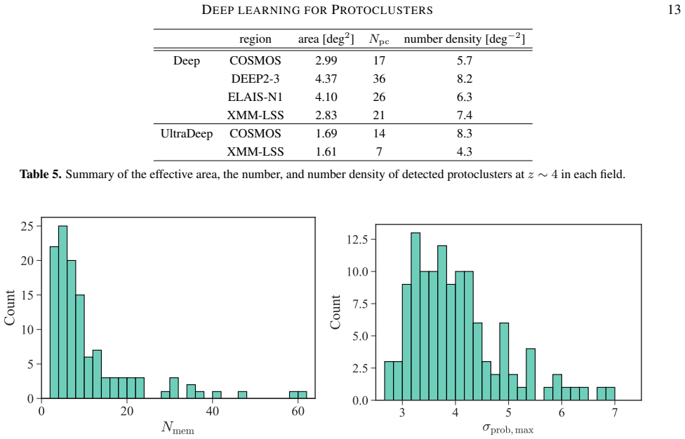
- [Section 5.2 and Table 5] The Deep and UltraDeep fields overlap on the sky (for example, COSMOS is listed as both Deep and UltraDeep), and the table entries sum to 121; please state explicitly whether the 121 candidates are merged across layers and whether 'unique' excludes objects detected in both layers.
- [Equation (13) and Section 5.2] The normalization of sigma_prob uses the mean and standard deviation of the evaluation data, which are then applied to HSC observations; please justify this choice given the known depth and number-density differences between Deep and UltraDeep, or explain how the domain shift is handled.
- [Section 4.2] The sentence introducing the grouping threshold as 'the minimum number of protocluster members, i.e., gamma N_th in case of lowest completeness' is unclear and should be rewritten for precision.
Circularity Check
Evaluation light cones share 13.7% of their galaxies with the training light cones, so the headline five-times-recall and low-mass-progenitor gains are measured on a non-independent evaluation set.
-
fitted input called prediction
[Section 2.1, 'Simualtion Data – PCcone', data-split paragraph]
"We note that the same galaxies may appear in training and validation/evaluation data because light cones are made from the same simulation boxes on Millennium Simulation. However, the input information (e.g., coordinates or magnitudes; see Sec 3.2) varies because the direction of the line of sight and the resampled magnitudes differ, and the possibility of critical overtraining or leakage is slight."
The headline performance claims (Sec. 4.1: recall = 7.5 +- 0.2%, precision = 44 +- 1%, five-fold and eleven-fold recall gains over 2DBM; Sec. 6.1: 7 +- 2 times more M_halo^z=0 < 10^15 Msun progenitors, and 23 versus 1 low-mass protoclusters) are computed on the four evaluation light cones. A large fraction of the evaluation galaxies (11264/82245 Deep, 10345/77986 UltraDeep) are the same simulated galaxies that appear in the 15 training light cones, so the network has already seen their halo environment and member/nonmember labels during training; only coordinates and resampled magnitudes differ.
full rationale
The derivation chain is not circular in the pure self-definitional sense: protocluster labels are independently defined from merger trees and descendant halo masses (Sec. 2.3), the 2DBM/3DBM baselines are independent methods, and the MDN redshift estimator is compared with EAZY on simulated truth. The dominant circularity risk is the training/evaluation overlap within PCcone. Because the four evaluation light cones are cut from the same Millennium Simulation box as the 15 training cones and share 11,264 (Deep) and 10,345 (UltraDeep) individual galaxies, the simulation-side precision/recall, PR AUC, and descendant-halo-mass distributions are not fully external validations. This directly undercuts the abstract's claim that PCFNet 'detects five times more protocluster member candidates' and the Sec. 6.1 claim that it detects 7 +- 2 times more low-mass progenitors. The observational application to HSC-SSP is an independent input, but it lacks spectroscopic ground truth; the only cross-check is spatial matching to Toshikawa et al. (2024), which is a consistency check rather than an external performance benchmark. Other weaknesses of the paper, such as the semi-analytic model not perfectly reproducing the real universe and the absence of spectroscopic confirmation for the 121 candidates, are correctness risks rather than circularity. Overall, the central simulation-based performance claim is partially circular because the evaluation set is not independent of the training set by construction, but the labels and baseline comparisons retain independent content, so the score is moderate rather than severe.
Assumptions & free parameters
free parameters (6)
- Protocluster member threshold N_th =
5
- Detection significance threshold sigma_th =
2.5
- MDN mixture components K =
3
- PCFNet training hyperparameters =
lr=0.001, batch size 512, dropout p=0.3
- Protocluster search aperture =
r=1.8 arcmin on a 1 arcmin grid
- Mask correction cubic function =
not given numerically
assumptions (6)
- domain assumption PCcone, built from the Millennium Simulation and L-GALAXIES, accurately reproduces the z~4 g-dropout galaxy population and HSC-SSP photometry.
- domain assumption Merger-tree main progenitor identification correctly defines protocluster cores and member galaxies at z=4.
- domain assumption The g-dropout selection of Eq. 1 isolates a representative z~4 galaxy population.
- domain assumption The MDN redshift probability density functions from g, r, i magnitudes contain enough line-of-sight information for PCFNet to separate protocluster members from foreground and background galaxies.
- domain assumption HSC-SSP photometric calibration, flags, and masking corrections preserve the feature distribution seen in the simulation.
- domain assumption The overlap of galaxies between training and evaluation light cones has a negligible effect on measured performance.
Cite this review
Pith. "Pith review of Mining for Protoclusters at $z\sim4$ from Photometric Datasets with Deep Learning." pith.science (2026). https://pith.science/paper/FLXMEP6L
@misc{pith2026241111956,
  author       = {Pith},
  title        = {Pith review of: Mining for Protoclusters at $z\sim4$ from Photometric Datasets with Deep Learning},
  year         = {2026},
  howpublished = {\url{https://pith.science/paper/FLXMEP6L}},
  note         = {Machine review of arXiv:2411.11956}
}
abstract
Protoclusters are high-$z$ overdense regions that will evolve into clusters of galaxies by $z=0$, making them ideal for studying galaxy evolution expected to be accelerated by environmental effects. However, it has been challenging to identify protoclusters beyond $z=3$ only by photometry due to large redshift uncertainties, hindering statistical study. To tackle the issue, we develop a new deep-learning-based protocluster detection model, PCFNet, which considers a protocluster as a point cloud. To detect protoclusters at $z\sim4$ using only optical broad-band photometry, we train and evaluate PCFNet with mock $g$-dropout galaxies based on the N-body simulation with the semi-analytic model. We use the sky distribution, $i$-band magnitude, $(g-i)$ color, and the redshift probability density function surrounding a target galaxy on the sky. PCFNet achieves to detect five times more protocluster member candidates while maintaining high purity (recall $=7.5\pm0.2$%, precision $=44\pm1$%) than conventional methods. Moreover, PCFNet is able to detect more progenitors ($M_\mathrm{halo}^{z=0}=10^{14-14.5}\,M_\odot$) that are less massive than supermassive clusters like the Coma cluster. We apply PCFNet to the observational photometric dataset of the HSC-SSP Deep/UltraDeep layer ($\sim17\mathrm{\,deg^2}$) and detect $121$ protocluster candidates at $z\sim4$. We find the rest-UV luminosities of our protocluster member candidates are brighter than those of field galaxies, which is consistent with previous studies. Additionally, the quenching of satellite galaxies depends on both the core galaxy's halo mass at $z\sim4$ and accumulated mass until $z=0$ in the simulation. PCFNet is very flexible and can find protoclusters at other redshifts or in future extensive surveys by Euclid, LSST, and Roman.
Figures


Figures from the paper (12 more)




Reference graph
Works this paper leans on
-
[1]
2020, ApJS, 249, 3, doi: 10.3847/1538-4365/ab929e
Ahumada, R., Allende Prieto, C., Almeida, A., et al. 2020, ApJS, 249, 3, doi: 10.3847/1538-4365/ab929e
-
[2]
2018, PASJ, 70, S8, doi: 10.1093/pasj/psx081
Aihara, H., Armstrong, R., Bickerton, S., et al. 2018, PASJ, 70, S8, doi: 10.1093/pasj/psx081
-
[3]
2022, PASJ, 74, 247, doi: 10.1093/pasj/psab122
Aihara, H., AlSayyad, Y ., Ando, M., et al. 2022, PASJ, 74, 247, doi: 10.1093/pasj/psab122
-
[4]
2022, arXiv e-prints, arXiv:2211.12346, doi: 10.48550/arXiv.2211.12346
Anagnostidis, S., Thomsen, A., Kacprzak, T., et al. 2022, arXiv e-prints, arXiv:2211.12346, doi: 10.48550/arXiv.2211.12346
-
[5]
2021, A&A, 650, A90, doi: 10.1051/0004-6361/202039675
Ansari, Z., Agnello, A., & Gall, C. 2021, A&A, 650, A90, doi: 10.1051/0004-6361/202039675
-
[6]
C., Sodré, Laerte, J., Overzier, R
Araya-Araya, P., Vicentin, M. C., Sodré, Laerte, J., Overzier, R. A., & Cuevas, H. 2021, MNRAS, 504, 5054, doi: 10.1093/mnras/stab1133 Astropy Collaboration, Robitaille, T. P., Tollerud, E. J., et al. 2013, A&A, 558, A33, doi: 10.1051/0004-6361/201322068 Astropy Collaboration, Price-Whelan, A. M., Sip˝ocz, B. M., et al. 2018, AJ, 156, 123, doi: 10.3847/15...
-
[7]
P., Jankowiak, M., et al
Bingham, E., Chen, J. P., Jankowiak, M., et al. 2019, J. Mach. Learn. Res., 20, 28:1. http://jmlr.org/papers/v20/18-403.html
2019
-
[8]
Bradshaw, E. J., Almaini, O., Hartley, W. G., et al. 2013, MNRAS, 433, 194, doi: 10.1093/mnras/stt715
Show all 118 references
-
[9]
B., van Dokkum, P
Brammer, G. B., van Dokkum, P. G., & Coppi, P. 2008, ApJ, 686, 1503, doi: 10.1086/591786
2008 doi
-
[10]
2021, MNRAS, 502, 4558, doi: 10.1093/mnras/staa4037
Calvi, R., Dannerbauer, H., Arrabal Haro, P., et al. 2021, MNRAS, 502, 4558, doi: 10.1093/mnras/staa4037
2021 doi
-
[11]
L., Hu, E
Capak, P., Cowie, L. L., Hu, E. M., et al. 2004, AJ, 127, 180, doi: 10.1086/380611
2004 doi
-
[12]
L., Riechers, D., Scoville, N
Capak, P. L., Riechers, D., Scoville, N. Z., et al. 2011, Nature, 470, 233, doi: 10.1038/nature09681
2011 doi
-
[13]
C., McLeod, D
Carnall, A. C., McLeod, D. J., McLure, R. J., et al. 2023, MNRAS, 520, 3974, doi: 10.1093/mnras/stad369
2023 doi
-
[14]
2022, A&A, 662, A115, doi: 10.1051/0004-6361/202243348
Castellano, M., Pentericci, L., Cupani, G., et al. 2022, A&A, 662, A115, doi: 10.1051/0004-6361/202243348
2022 doi
-
[15]
2023, MNRAS, doi: 10.1093/mnras/stad1868
Chen, X., Zhu, F., Gaines, S., & Padmanabhan, N. 2023, MNRAS, doi: 10.1093/mnras/stad1868
2023 doi
-
[16]
2013, ApJ, 779, 127, doi: 10.1088/0004-637X/779/2/127
Chiang, Y .-K., Overzier, R., & Gebhardt, K. 2013, ApJ, 779, 127, doi: 10.1088/0004-637X/779/2/127
2013 doi
-
[17]
A., Gebhardt, K., & Henriques, B
Chiang, Y .-K., Overzier, R. A., Gebhardt, K., & Henriques, B. 2017, ApJL, 844, L23, doi: 10.3847/2041-8213/aa7e7b
2017 doi
-
[18]
L., Blanton, M
Coil, A. L., Blanton, M. R., Burles, S. M., et al. 2011, ApJ, 741, 8, doi: 10.1088/0004-637X/741/1/8
2011 doi
- [19]
-
[20]
Conroy, C., & Gunn, J. E. 2010, ApJ, 712, 833, doi: 10.1088/0004-637X/712/2/833
2010 doi
-
[21]
E., & White, M
Conroy, C., Gunn, J. E., & White, M. 2009, ApJ, 699, 486, doi: 10.1088/0004-637X/699/1/486
2009 doi
-
[22]
A., Hatch, N
Cooke, E. A., Hatch, N. A., Rettura, A., et al. 2015, MNRAS, 452, 2318, doi: 10.1093/mnras/stv1413
2015 doi
-
[23]
J., Moustakas, J., Blanton, M
Cool, R. J., Moustakas, J., Blanton, M. R., et al. 2013, ApJ, 767, 118, doi: 10.1088/0004-637X/767/2/118
2013 doi
-
[24]
C., Aird, J
Cooper, M. C., Aird, J. A., Coil, A. L., et al. 2011, ApJS, 193, 14, doi: 10.1088/0067-0049/193/1/14
2011 doi
-
[26]
M., Newman, J., et al
Davis, M., Faber, S. M., Newman, J., et al. 2003, in Society of Photo-Optical Instrumentation Engineers (SPIE) Conference
2003
-
[27]
4834, Discoveries and Research Prospects from 6- to 10-Meter-Class Telescopes II, ed
Series, V ol. 4834, Discoveries and Research Prospects from 6- to 10-Meter-Class Telescopes II, ed. P. Guhathakurta, 161–172, doi: 10.1117/12.457897 De Lucia, G., & Blaizot, J. 2007, MNRAS, 375, 2, doi: 10.1111/j.1365-2966.2006.11287.x Di Matteo, T., Springel, V ., & Hernquist...
2007
-
[28]
1980, ApJ, 236, 351, doi: 10.1086/157753
Dressler, A. 1980, ApJ, 236, 351, doi: 10.1086/157753
1980 doi
-
[30]
Endsley, R., & Stark, D. P. 2022, MNRAS, 511, 6042, doi: 10.1093/mnras/stac524
2022 doi
-
[32]
2008, ApJS, 176, 1, doi: 10.1086/527321 Ganeshaiah Veena, P., Lilow, R., & Nusser, A
Furusawa, H., Kosugi, G., Akiyama, M., et al. 2008, ApJS, 176, 1, doi: 10.1086/527321 Ganeshaiah Veena, P., Lilow, R., & Nusser, A. 2023, MNRAS, 522, 5291, doi: 10.1093/mnras/stad1222
2008 doi
-
[33]
2014, A&A, 562, A23, doi: 10.1051/0004-6361/201322790
Garilli, B., Guzzo, L., Scodeggio, M., et al. 2014, A&A, 562, A23, doi: 10.1051/0004-6361/201322790
2014 doi
-
[34]
2012, in 2012 IEEE conference on computer vision and pattern recognition, IEEE, 3354–3361
Geiger, A., Lenz, P., & Urtasun, R. 2012, in 2012 IEEE conference on computer vision and pattern recognition, IEEE, 3354–3361
2012
-
[35]
Glorot, X., Bordes, A., & Bengio, Y . 2011, in Proceedings of the fourteenth international conference on artificial intelligence and statistics, JMLR Workshop and Conference Proceedings, 315–323 Gottlöber, S., Klypin, A., & Kravtsov, A. V . 2001, ApJ, 546, 223, doi: 10.1086/318248
2011 doi
-
[36]
2019, ApJ, 883, 142, doi: 10.3847/1538-4357/ab2cd5
Harikane, Y ., Ouchi, M., Ono, Y ., et al. 2019, ApJ, 883, 142, doi: 10.3847/1538-4357/ab2cd5
2019 doi
-
[37]
R., Millman, K
Harris, C. R., Millman, K. J., van der Walt, S. J., et al. 2020, Nature, 585, 357, doi: 10.1038/s41586-020-2649-2
2020 doi
-
[38]
2023, ApJL, 955, L2, doi: 10.3847/2041-8213/acf57c
Hashimoto, T., Álvarez-Márquez, J., Fudamoto, Y ., et al. 2023, ApJL, 955, L2, doi: 10.3847/2041-8213/acf57c
2023 doi
-
[39]
2018, ApJ, 858, 77, doi: 10.3847/1538-4357/aabacf
Hasinger, G., Capak, P., Salvato, M., et al. 2018, ApJ, 858, 77, doi: 10.3847/1538-4357/aabacf
2018 doi
-
[40]
A., Kurk, J
Hatch, N. A., Kurk, J. D., Pentericci, L., et al. 2011, MNRAS, 415, 2993, doi: 10.1111/j.1365-2966.2011.18735.x
2011
-
[41]
M., Sun, F., Woodrum, C., et al
Helton, J. M., Sun, F., Woodrum, C., et al. 2024, ApJ, 962, 124, doi: 10.3847/1538-4357/ad0da7
2024 doi
-
[42]
Henriques, B. M. B., White, S. D. M., Thomas, P. A., et al. 2015, MNRAS, 451, 2663, doi: 10.1093/mnras/stv705
2015 doi
-
[43]
F., Cox, T
Hopkins, P. F., Cox, T. J., Kereš, D., & Hernquist, L. 2008, ApJS, 175, 390, doi: 10.1086/524363
2008 doi
-
[44]
2021, Nature Astronomy, 5, 485, doi: 10.1038/s41550-020-01291-y
Hu, W., Wang, J., Infante, L., et al. 2021, Nature Astronomy, 5, 485, doi: 10.1038/s41550-020-01291-y
2021 doi
-
[45]
Hunter, J. D. 2007, Computing in Science & Engineering, 9, 90, doi: 10.1109/MCSE.2007.55
2007 doi
-
[46]
2022, MNRAS, 515, 4065, doi: 10.1093/mnras/stac2055
Inoue, S., Si, X., Okamoto, T., & Nishigaki, M. 2022, MNRAS, 515, 4065, doi: 10.1093/mnras/stac2055
2022 doi
-
[47]
2016, ApJ, 822, 5, doi: 10.3847/0004-637X/822/1/5
Ishigaki, M., Ouchi, M., & Harikane, Y . 2016, ApJ, 822, 5, doi: 10.3847/0004-637X/822/1/5
2016 doi
-
[48]
2020, ApJ, 899, 5, doi: 10.3847/1538-4357/aba269
Ito, K., Kashikawa, N., Toshikawa, J., et al. 2020, ApJ, 899, 5, doi: 10.3847/1538-4357/aba269
2020 doi
-
[49]
2021, ApJ, 916, 35, doi: 10.3847/1538-4357/abfc50
Ito, K., Kashikawa, N., Tanaka, M., et al. 2021, ApJ, 916, 35, doi: 10.3847/1538-4357/abfc50
2021 doi
-
[50]
2023, ApJL, 945, L9, doi: 10.3847/2041-8213/acb49b Ivezi´c, Ž., Kahn, S
Ito, K., Tanaka, M., Valentino, F., et al. 2023, ApJL, 945, L9, doi: 10.3847/2041-8213/acb49b Ivezi´c, Ž., Kahn, S. M., Tyson, J. A., et al. 2019, ApJ, 873, 111, doi: 10.3847/1538-4357/ab042c
2023 doi
-
[51]
H., Saunders, W., Colless, M., et al
Jones, D. H., Saunders, W., Colless, M., et al. 2004, MNRAS, 355, 747, doi: 10.1111/j.1365-2966.2004.08353.x
2004
-
[52]
H., Read, M
Jones, D. H., Read, M. A., Saunders, W., et al. 2009, MNRAS, 399, 683, doi: 10.1111/j.1365-2966.2009.15338.x
2009
-
[53]
S., Daddi, E., Bournaud, F., et al
Kalita, B. S., Daddi, E., Bournaud, F., et al. 2022, A&A, 666, A44, doi: 10.1051/0004-6361/202243100 Kereš, D., Katz, N., Weinberg, D. H., & Davé, R. 2005, MNRAS, 363, 2, doi: 10.1111/j.1365-2966.2005.09451.x
2022
- [54]
-
[55]
D., Faber, S
Kocevski, D. D., Faber, S. M., Mozena, M., et al. 2012, ApJ, 744, 148, doi: 10.1088/0004-637X/744/2/148
2012 doi
-
[56]
2012, ApJL, 746, L22, doi: 10.1088/2041-8205/746/2/L22
Koss, M., Mushotzky, R., Treister, E., et al. 2012, ApJL, 746, L22, doi: 10.1088/2041-8205/746/2/L22
2012 doi
-
[57]
2013, MNRAS, 428, 1551, doi: 10.1093/mnras/sts133
Koyama, Y ., Kodama, T., Tadaki, K.-i., et al. 2013, MNRAS, 428, 1551, doi: 10.1093/mnras/sts133
2013 doi
-
[58]
2018, ApJ, 867, 1, doi: 10.3847/1538-4357/aae3e8
Kubo, M., Tanaka, M., Yabe, K., et al. 2018, ApJ, 867, 1, doi: 10.3847/1538-4357/aae3e8
2018 doi
-
[59]
2019, ApJ, 887, 214, doi: 10.3847/1538-4357/ab5a80
Kubo, M., Toshikawa, J., Kashikawa, N., et al. 2019, ApJ, 887, 214, doi: 10.3847/1538-4357/ab5a80
2019 doi
-
[60]
2022, ApJ, 935, 89, doi: 10.3847/1538-4357/ac7f2d
Kubo, M., Umehata, H., Matsuda, Y ., et al. 2022, ApJ, 935, 89, doi: 10.3847/1538-4357/ac7f2d
2022 doi
-
[61]
1993, MNRAS, 262, 627, doi: 10.1093/mnras/262.3.627
Lacey, C., & Cole, S. 1993, MNRAS, 262, 627, doi: 10.1093/mnras/262.3.627
1993 doi
-
[62]
L., Finkelstein, S
Larson, R. L., Finkelstein, S. L., Hutchison, T. A., et al. 2022, ApJ, 930, 104, doi: 10.3847/1538-4357/ac5dbd Le Fèvre, O., Cassata, P., Cucciati, O., et al. 2013, A&A, 559, A14, doi: 10.1051/0004-6361/201322179
2022 doi
-
[63]
Lebigot, E. O. 2016, Uncertainties: a Python package for calculations with uncertainties. http://pythonhosted.org/uncertainties/
2016
-
[64]
2006, in Astronomical Society of the Pacific Conference Series, V ol
Lemson, G., & Springel, V . 2006, in Astronomical Society of the Pacific Conference Series, V ol. 351, Astronomical Data Analysis Software and Systems XV , ed. C. Gabriel, C. Arviset, D. Ponz, & S. Enrique, 212
2006
-
[65]
2002, MNRAS, 334, 673, doi: 10.1046/j.1365-8711.2002.05558.x
Lewis, I., Balogh, M., De Propris, R., et al. 2002, MNRAS, 334, 673, doi: 10.1046/j.1365-8711.2002.05558.x
2002
-
[66]
J., Le Brun, V ., Maier, C., et al
Lilly, S. J., Le Brun, V ., Maier, C., et al. 2009, ApJS, 184, 218, doi: 10.1088/0067-0049/184/2/218
2009 doi
-
[67]
2021, MNRAS, 501, 1803, doi: 10.1093/mnras/staa3693
Lim, S., Scott, D., Babul, A., et al. 2021, MNRAS, 501, 1803, doi: 10.1093/mnras/staa3693
2021 doi
- [68]
-
[69]
K., Driver, S
Liske, J., Baldry, I. K., Driver, S. P., et al. 2015, MNRAS, 452, 2087, doi: 10.1093/mnras/stv1436 maintainers, T., & contributors. 2016, TorchVision: PyTorch’s Computer Vision library, https://github.com/pytorch/vision, GitHub
2015 doi
-
[70]
C., Muzzin, A., Marchesini, D., et al
Marsan, Z. C., Muzzin, A., Marchesini, D., et al. 2022, ApJ, 924, 25, doi: 10.3847/1538-4357/ac312a
2022 doi
-
[71]
C., Stern, D
Masters, D. C., Stern, D. K., Cohen, J. G., et al. 2017, ApJ, 841, 111, doi: 10.3847/1538-4357/aa6f08 —. 2019, ApJ, 877, 81, doi: 10.3847/1538-4357/ab184d
2017 doi
-
[72]
2022, ApJ, 926, 37, doi: 10.3847/1538-4357/ac2b9f
McConachie, I., Wilson, G., Forrest, B., et al. 2022, ApJ, 926, 37, doi: 10.3847/1538-4357/ac2b9f
2022 doi
-
[73]
J., Pearce, H
McLure, R. J., Pearce, H. J., Dunlop, J. S., et al. 2013, MNRAS, 428, 1088, doi: 10.1093/mnras/sts092
2013 doi
-
[74]
A., et al
Mechtley, M., Jahnke, K., Windhorst, R. A., et al. 2016, ApJ, 830, 156, doi: 10.3847/0004-637X/830/2/156
2016 doi
-
[75]
B., Chapman, S
Miller, T. B., Chapman, S. C., Aravena, M., et al. 2018, Nature, 556, 469, doi: 10.1038/s41586-018-0025-2
2018 doi
-
[76]
G., Brammer, G
Momcheva, I. G., Brammer, G. B., van Dokkum, P. G., et al. 2016, ApJS, 225, 27, doi: 10.3847/0067-0049/225/2/27
2016 doi
-
[77]
2023, ApJL, 947, L24, doi: 10.3847/2041-8213/acb99e
Morishita, T., Roberts-Borsani, G., Treu, T., et al. 2023, ApJL, 947, L24, doi: 10.3847/2041-8213/acb99e
2023 doi
-
[78]
I., Hatch, N
Muldrew, S. I., Hatch, N. A., & Cooke, E. A. 2015, MNRAS, 452, 2528, doi: 10.1093/mnras/stv1449 —. 2018, MNRAS, 473, 2335, doi: 10.1093/mnras/stx2454
2015 doi
-
[79]
A., Cooper, M
Newman, J. A., Cooper, M. C., Davis, M., et al. 2013, ApJS, 208, 5, doi: 10.1088/0067-0049/208/1/5
2013 doi
- [80]
-
[81]
2008, MNRAS, 390, 1326, doi: 10.1111/j.1365-2966.2008.13763.x
Ocvirk, P., Pichon, C., & Teyssier, R. 2008, MNRAS, 390, 1326, doi: 10.1111/j.1365-2966.2008.13763.x
2008
- [82]
-
[83]
J., Balogh, M
Old, L. J., Balogh, M. L., van der Burg, R. F. J., et al. 2020, MNRAS, 493, 5987, doi: 10.1093/mnras/staa579
2020 doi
-
[84]
2018, PASJ, 70, S10, doi: 10.1093/pasj/psx103
Ono, Y ., Ouchi, M., Harikane, Y ., et al. 2018, PASJ, 70, S10, doi: 10.1093/pasj/psx103
2018 doi
-
[85]
2018, PASJ, 70, S31, doi: 10.1093/pasj/psx092
Onoue, M., Kashikawa, N., Uchiyama, H., et al. 2018, PASJ, 70, S31, doi: 10.1093/pasj/psx092
2018 doi
-
[86]
J., Dunne, L., et al
Oteo, I., Ivison, R. J., Dunne, L., et al. 2018, ApJ, 856, 72, doi: 10.3847/1538-4357/aaa1f1
2018 doi
- [87]
- [88]
-
[89]
2011, Journal of Machine Learning Research, 12, 2825 Planck Collaboration, Ade, P
Pedregosa, F., Varoquaux, G., Gramfort, A., et al. 2011, Journal of Machine Learning Research, 12, 2825 Planck Collaboration, Ade, P. A. R., Aghanim, N., et al. 2014, A&A, 571, A16, doi: 10.1051/0004-6361/201321591
2011 doi
-
[90]
Postman, M., & Geller, M. J. 1984, ApJ, 281, 95, doi: 10.1086/162078
1984 doi
- [91]
-
[92]
2023, ApJ, 950, 191, doi: 10.3847/1538-4357/accb91
Remus, R.-S., Dolag, K., & Dannerbauer, H. 2023, ApJ, 950, 191, doi: 10.3847/1538-4357/accb91
2023 doi
-
[93]
A., Kartaltepe, J
Shah, E. A., Kartaltepe, J. S., Magagnoli, C. T., et al. 2020, ApJ, 904, 107, doi: 10.3847/1538-4357/abbf59
2020 doi
-
[94]
A., Lemaux, B., Forrest, B., et al
Shah, E. A., Lemaux, B., Forrest, B., et al. 2024, MNRAS, 529, 873, doi: 10.1093/mnras/stae519
2024 doi
-
[95]
Shimakawa, R., Koyama, Y ., Röttgering, H. J. A., et al. 2018, MNRAS, 481, 5630, doi: 10.1093/mnras/sty2618
2018 doi
-
[96]
B., Jin, S., Magdis, G
Sillassen, N. B., Jin, S., Magdis, G. E., et al. 2022, A&A, 665, L7, doi: 10.1051/0004-6361/202244661
2022 doi
-
[97]
D., Kashino, D., Sanders, D., et al
Silverman, J. D., Kashino, D., Sanders, D., et al. 2015, ApJS, 220, 12, doi: 10.1088/0067-0049/220/1/12
2015 doi
-
[98]
E., Whitaker, K
Skelton, R. E., Whitaker, K. E., Momcheva, I. G., et al. 2014, ApJS, 214, 24, doi: 10.1088/0067-0049/214/2/24
2014 doi
-
[99]
S., & White, S
Springel, V ., Frenk, C. S., & White, S. D. M. 2006, Nature, 440, 1137, doi: 10.1038/nature04805
2006 doi
-
[100]
C., Forrest, B., et al
Staab, P., Lemaux, B. C., Forrest, B., et al. 2024, MNRAS, 528, 6934, doi: 10.1093/mnras/stae301
2024 doi
-
[101]
Adelberger, K. L. 1996, ApJL, 462, L17, doi: 10.1086/310029
1996 doi
-
[102]
Straatman, C. M. S., van der Wel, A., Bezanson, R., et al. 2018, ApJS, 239, 27, doi: 10.3847/1538-4365/aae37a
2018 doi
-
[103]
T., Daddi, E., et al
Strazzullo, V ., Coogan, R. T., Daddi, E., et al. 2018, ApJ, 862, 64, doi: 10.3847/1538-4357/aacd10
2018 doi
- [104]
-
[105]
2020, findpeaks is for the detection of peaks and valleys in a 1D vector and 2D array (image)., 2.3.1
Taskesen, E. 2020, findpeaks is for the detection of peaks and valleys in a 1D vector and 2D array (image)., 2.3.1. https://erdogant.github.io/findpeaks
2020
-
[106]
2005, ApJ, 621, 673, doi: 10.1086/426932
Thomas, D., Maraston, C., Bender, R., & Mendes de Oliveira, C. 2005, ApJ, 621, 673, doi: 10.1086/426932
2005 doi
-
[107]
2012, ApJ, 750, 137, doi: 10.1088/0004-637X/750/2/137
Toshikawa, J., Kashikawa, N., Ota, K., et al. 2012, ApJ, 750, 137, doi: 10.1088/0004-637X/750/2/137
2012 doi
-
[108]
2018, PASJ, 70, S12, doi: 10.1093/pasj/psx102
Toshikawa, J., Uchiyama, H., Kashikawa, N., et al. 2018, PASJ, 70, S12, doi: 10.1093/pasj/psx102
2018 doi
-
[109]
2024, MNRAS, 527, 6276, doi: 10.1093/mnras/stad3162
Toshikawa, J., Wuyts, S., Kashikawa, N., et al. 2024, MNRAS, 527, 6276, doi: 10.1093/mnras/stad3162
2024 doi
-
[110]
D., Stiavelli, M., et al
Trenti, M., Bradley, L. D., Stiavelli, M., et al. 2012, ApJ, 746, 55, doi: 10.1088/0004-637X/746/1/55
2012 doi
-
[111]
2018, PASJ, 70, S32, doi: 10.1093/pasj/psx112
Uchiyama, H., Toshikawa, J., Kashikawa, N., et al. 2018, PASJ, 70, S32, doi: 10.1093/pasj/psx112
2018 doi
-
[112]
2020, ApJ, 905, 125, doi: 10.3847/1538-4357/abc47b 22 T AKEDA ET AL
Uchiyama, H., Akiyama, M., Toshikawa, J., et al. 2020, ApJ, 905, 125, doi: 10.3847/1538-4357/abc47b 22 T AKEDA ET AL
2020 doi
-
[113]
Valentino, F., Brammer, G., Gould, K. M. L., et al. 2023, ApJ, 947, 20, doi: 10.3847/1538-4357/acbefa van der Burg, R. F. J., Rudnick, G., Balogh, M. L., et al. 2020, A&A, 638, A112, doi: 10.1051/0004-6361/202037754
2023 doi
-
[114]
E., et al
Virtanen, P., Gommers, R., Oliphant, T. E., et al. 2020, Nature Methods, 17, 261, doi: 10.1038/s41592-019-0686-2
2020 doi
-
[115]
2012, Nature, 486, 233, doi: 10.1038/nature11073
Walter, F., Decarli, R., Carilli, C., et al. 2012, Nature, 486, 233, doi: 10.1038/nature11073
2012 doi
-
[116]
F., et al
Wang, F., Yang, J., Hennawi, J. F., et al. 2024, ApJL, 962, L11, doi: 10.3847/2041-8213/ad20ef
2024 doi
-
[117]
2018a, ApJL, 867, L29, doi: 10.3847/2041-8213/aaeb2c
Wang, T., Elbaz, D., Daddi, E., et al. 2018a, ApJL, 867, L29, doi: 10.3847/2041-8213/aaeb2c
-
[118]
2018b, arXiv e-prints, arXiv:1801.07829, doi: 10.48550/arXiv.1801.07829 Wes McKinney
Wang, Y ., Sun, Y ., Liu, Z., et al. 2018b, arXiv e-prints, arXiv:1801.07829, doi: 10.48550/arXiv.1801.07829 Wes McKinney. 2010, in Proceedings of the 9th Python in Science Conference, ed. Stéfan van der Walt & Jarrod Millman, 56 – 61, doi: 10.25080/Majora-92bf1922-00a
- [119]
-
[120]
2023, MNRAS, 522, 4748, doi: 10.1093/mnras/stad1290
Wu, Z., Xiao, L., Xiao, X., et al. 2023, MNRAS, 522, 4748, doi: 10.1093/mnras/stad1290
2023 doi
-
[121]
2022, MNRAS, 509, 4037, doi: 10.1093/mnras/stab3092
Yajima, H., Abe, M., Khochfar, S., et al. 2022, MNRAS, 509, 4037, doi: 10.1093/mnras/stab3092
2022 doi
Reviewed August 12, 2026 · model on record in the stance chip above.
Discussion (0). Continue with ORCID to comment.