REVIEW 4 major objections 4 minor 69 references
LC-SVD-DLinear: A low-cost physics-based hybrid machine learning model for data forecasting using sparse measurements
T0 review · 4 major / 4 minor · reviewed 2026-08-12 · deepseek-v4-flash
Pith's one-line read A hybrid model combining low-cost singular value decomposition with the DLinear network can forecast high-resolution fluid flow snapshots from under-resolved or sparse measurements, with reconstruction errors as low as 0.571% on a laminar…
desk verdict The pipeline is coherent and LC-HOSVD is a real extension, but the headline test errors aren't clean out-of-sample because the spatial basis is fit to the full dataset, so the forecasting claim is over-supported. read the letter →
The pith
A machine-rendered reading of the paper's core claim, the machinery that carries it, and where it could break.
The reading
What carries the argument
The load-bearing object is the reconstructed spatial modes matrix $W^{\mathrm{rec}}$ together with the reconstructed temporal coefficients $T^{\mathrm{rec}}$, obtained from an under-resolved snapshot matrix by the LC-SVD reconstruction formulas (Eqs. 2.12-2.14). The temporal coefficients are then decomposed by DLinear into trend and seasonality using an average-pooling layer, forecast autoregressively with one linear layer per component, and recombined as $\hat{V} = W^{\mathrm{rec}} \bar{\Sigma} (\hat{T}^{\mathrm{rec}})^\top$ to form new snapshots. LC-HOSVD applies a component-wise tensor decomposition before the same LC-SVD reconstruction, allowing mode filtering per spatial component.
What would settle it
Run the pipeline on a flow that undergoes a controlled change of regime after the training window, such as a cylinder wake with a sudden Reynolds-number change or an oncoming gust, and measure the RRMSE of the forecast snapshots against a full simulation. If the error grows sharply when the new coherent structure appears, that confirms the fixed-basis assumption is the limiting factor; if the error stays near the reported 0.5-12% levels, the basis is more transferable than assumed.
Extended reading notes
Core claim
The central discovery is that the temporal coefficients produced by a low-cost SVD or HOSVD reconstruction form a smooth, low-dimensional time series that a simple linear decomposition network can forecast accurately, and that this forecast can be lifted back to full spatial resolution using the reconstructed spatial modes. LC-SVD reconstructs the spatial modes $W^{\mathrm{rec}}$ and temporal coefficients $T^{\mathrm{rec}}$ from under-resolved data using Eqs. (2.12)-(2.14); DLinear splits $T^{\mathrm{rec}}$ into trend and seasonality via an average-pooling decomposition, forecasts each component with one linear layer per mode, and the autoregressive predictions are recombined with $W^{\mathrm{rec}}$ and the singular values to form future snapshots. LC-HOSVD performs a component-wise tensor decomposition before the same reconstruction step, which the paper finds gives cleaner mode filtering and slightly lower reconstruction errors.
Load-bearing premise
The pipeline assumes that the high-resolution spatial modes $W^{\mathrm{rec}}$ learned from paired training data remain a valid basis for the future snapshots being forecast; if the flow's coherent structures change after the training window, those modes cannot represent the new snapshots and the forecast error will grow regardless of how well the temporal coefficients are predicted.
Editorial extensions
If this is right
- Forecasts of 1000 snapshots for the laminar wake and 200 for the turbulent wake are generated from input sequences of length 15 and 100, respectively, with no visible drift in the velocity range.
- Because the computation happens on 45 or 40 sensor points instead of the full mesh, the forecast step is cheap regardless of the output resolution.
- The method works on both numerical and experimental data, and on both laminar and turbulent flows.
- LC-HOSVD-DLinear gives lower reconstruction error than LC-SVD-DLinear in both test cases: 0.571% versus 1.384% for the laminar wake and 10.571% versus 11.554% for the turbulent wake.
- For turbulent data, the paper reports that accuracy drops as more modes are retained, so the pipeline relies on keeping only a few robust modes.
Reading between the lines
- Editorial extension: because the fixed spatial basis is built from paired training data, the method should be most trustworthy while the flow's coherent structures remain unchanged; a flow that changes topology after the training window would likely produce growing forecast error.
- Editorial extension: the same pipeline could be tested on other quasi-periodic flows, such as flapping wings or bluff bodies at different Reynolds numbers, where DLinear's trend-seasonality decomposition should be able to exploit the periodic temporal coefficients.
- Editorial extension: an explicit comparison against training DLinear directly on full-resolution data, or against a recurrent network on the same temporal coefficients, would isolate how much of the accuracy comes from the SVD compression and denoising and how much from the linear forecaster.
- Editorial extension: the reported compression ratios (17,066 and 835) suggest that the forecast stage's memory cost is dominated by the number of retained modes, so the method should scale to larger three-dimensional meshes as long as the mode count stays small.
Signed reviews
Editorial analysis
A structured set of objections, weighed in public.
Referee Report
Summary. The paper introduces LC-SVD-DLinear and LC-HOSVD-DLinear, hybrid reduced-order models that combine low-cost singular value decomposition (or its higher-order variant) with the DLinear neural architecture. The pipeline decomposes an under-resolved dataset into spatial modes and temporal coefficients, uses DLinear to forecast the temporal coefficients autoregressively, and then reconstructs high-resolution snapshots by multiplying the forecast coefficients by reconstructed spatial modes. The method is demonstrated on a three-dimensional laminar cylinder wake at Re=220 and an experimental turbulent cylinder wake at Re=2600, with reported test reconstruction errors of RRMSE=1.384% and 0.571% for the laminar case and 11.554% and 10.571% for the turbulent case using LC-SVD-DLinear and LC-HOSVD-DLinear, respectively. The paper also presents extended forecasts of 1000 (laminar) and 200 (turbulent) snapshots and states that the approach provides uncertainty quantification and low computational cost.
Significance. If the evidence were fully out-of-sample, the proposed hybrid approach would be a useful contribution to sparse-sensor flow forecasting: the combination of LC-SVD/LC-HOSVD with a lightweight linear forecaster is sensible, the DLinear temporal extrapolation is a genuine held-out forecast of the temporal coefficients, and the LC-HOSVD variant appears to be new. The reported low reconstruction errors on the test sets would support the central claim of forecasting high-resolution snapshots from sparse measurements. However, as presented, the headline test errors are weakened by a basis-leakage issue, the abstract's promise of uncertainty quantification is not fulfilled, the extended forecasts are only visually assessed, and no runtime or baseline comparisons support the 'low-cost' claim. These issues are fixable within the scope of the manuscript, so the underlying idea remains viable after revision.
major comments (4)
- [§2.4 and Eq. (2.12)] The reported test-set RRMSE values are not out-of-sample evidence for forecasting because the spatial modes W_rec are computed from the entire input dataset before the train/validation/test split. Section 2.4 states that the temporal coefficients are split only after LC-SVD has reconstructed the spatial modes and temporal coefficients, and Eq. (2.12) constructs W_rec from the full snapshot matrix. Consequently, the spatial structure of the test-period snapshots has already informed W_rec, and the test reconstruction is a projection onto a basis that has seen those snapshots. This is especially consequential for the turbulent case, where only 6 modes are retained. The authors should recompute W_rec and T_rec using only the training snapshots, freeze those quantities, and then reconstruct the held-out test snapshots; only then would the reported RRMSEs (1.384%, 0.571%, 11.554%, 10.571%) validate the forecasting claim.
- [Abstract and §2.7/§4] The abstract promises that the forecasting and reconstruction results are evaluated 'including uncertainty quantification,' but no uncertainty intervals, confidence bands, ensemble statistics, or any other UQ tool appears in the error-analysis section or in the results. All reported errors are single point estimates (e.g., MAE=0.454, RRMSE=1.384%, Wasserstein distance at a single snapshot). If uncertainty quantification is part of the contribution, the manuscript must define how intervals are constructed and report them for the test-set reconstructions; otherwise the abstract should be revised to not promise UQ.
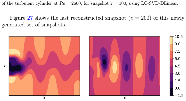
- [§4.1 and §4.2, extended forecasts] The multi-step forecasting capability is not quantitatively validated. The extended forecasts (Nsnap=1000 for the laminar case, Nsnap=200 for the turbulent case) are supported only by visual inspection of selected snapshots (Figs. 12-13, 19-20, 26-27, 33-34) and qualitative statements that velocity ranges remain stable. No error metric is reported for these extrapolated snapshots against any ground truth. Because the central claim includes forecasting many steps ahead, the authors should provide quantitative error measures on a held-out portion of the data, or clearly state that these extended forecasts are illustrative and not error-assessed.
- [§1 and §4, computational-cost claim] The 'low computational cost' part of the central claim is asserted but not measured for the hybrid pipeline. The paper cites speedups for LC-SVD from Ref. [56] but reports no runtime, memory, or FLOP comparisons for LC-SVD-DLinear or LC-HOSVD-DLinear against standard SVD/HOSVD, against DLinear applied directly to full-resolution data, or against a POD-DLinear baseline. Without such measurements, the reader cannot verify the claimed cost advantage. Adding a small benchmark table with training time, inference time, and memory for the full pipelines would directly support the paper's central claim.
minor comments (4)
- [§2.2, Eqs. (2.12)-(2.13)] The notation in Eqs. (2.12) and (2.13) is ambiguous: the superscripts on the snapshot matrix are not clearly defined, and it is not specified whether the reconstruction uses the low-resolution snapshot matrix or a paired high-resolution snapshot matrix. Please clarify the dimensions and state explicitly which data matrix is used in each equation.
- [§5 and §4] The conclusions state that 'the effects of the number of retained modes on the models performance accuracy has also been tested,' but no such sensitivity experiment appears in Section 4. Either add the experiment or remove the claim from the conclusions.
- [Various] There are several cross-reference errors and typos: the text refers to 'test data predictions in fig. 12 and fig. 19' where it likely means Figs. 9 and 16; the turbulent HOSVD subsection refers to 'fig. 26' and '27' where it means Figs. 33 and 34; 'Hofp bifurcation' should be 'Hopf bifurcation'; 'sings' in Section 2.2 should be 'signs'; and 'M SE' should be 'MSE.'
- [Abstract and §2.5] The abstract says DLinear enables the model to 'capture the non-linear dynamics of the temporal data,' but DLinear is a linear model. Please clarify that the nonlinearity comes from the decomposition and the autoregressive rolling-window loop, not from the linear layers themselves.
Circularity Check
Test-set snapshot 'predictions' reuse a spatial basis computed from the full dataset including the test period, so the headline RRMSE values are partly in-sample reconstruction rather than out-of-sample forecasting.
-
self definitional
[Sec. 2.2 Steps 4-6 (Eqs. 2.12-2.14); Sec. 2.4; Secs. 4.1-4.2]
"First, the input temporal coefficients matrix is divided into train, validation and test sets, with proportions 0.7, 0.15 and 0.15, respectively. ... W ≃ W rec = ( ¯V K,J ¯K 1 )⊤ ¯T ( ¯Σ)−1, where W rec ∈ RJ× ¯N . ... V K 1 ≃ V K,rec 1 = W rec ¯Σ (T rec)⊤. ... The forecast temporal modes are used to reconstruct the test snapshots, with a reconstruction error of RRM SE= 1.384%."
Eqs. (2.12)-(2.14) compute the reconstruction basis W_rec (and the target temporal coefficients T_rec) from the entire snapshot matrix V^K_1; only afterward does Sec. 2.4 split the temporal coefficients into train/validation/test. Thus W_rec is the optimal rank-N spatial basis for the full dataset, including the very test snapshots whose 'forecast' is later evaluated. Reconstructing a test snapshot as W_rec Σ T_forecast^T projects it onto a basis learned from that same snapshot. If the DLinear temporal forecast were perfect, the reported test RRMSE would collapse to the rank-N SVD truncation error of the test data; the spatial part of the prediction is therefore in-sample by construction.
full rationale
The DLinear stage is a genuine autoregressive extrapolation of temporal coefficients, and no equation reduces the temporal forecast to a fitted target. Self-citations to [56] for LC-SVD and for the sensor counts are not themselves circular: they invoke prior work used as a component, not a uniqueness theorem or an ansatz smuggled in by citation. The significant circularity is in the evaluation protocol: the spatial SVD modes W_rec are computed from the whole dataset, including the test period, before the train/validation/test split is applied (Sec. 2.4), so the reported test-set snapshot errors are partly in-sample reconstruction of the test data. Because the paper's headline evidence for the central claim is these RRMSE values, the central claim is partially circular but not fully: the temporal coefficients are still forecast out-of-sample, so the method has independent content. Score 6 reflects one prediction component reducing, by construction, to a basis fitted to the target period.
Assumptions & free parameters
free parameters (6)
- Number of retained SVD/HOSVD modes (Nbar) =
12 (laminar), 6 (turbulent)
- Number of sensors (Ns) =
45 (laminar), 40 (turbulent)
- Sequence length (L) =
15 (laminar), 100 (turbulent)
- Learning rate (alpha) =
6.23e-4, 1.013e-4 (LC-SVD); 2.1e-4, 1.35e-4 (LC-HOSVD)
- Batch size (Bs) =
16/4 (LC-SVD), 4/4 (LC-HOSVD)
- Iterative reconstruction threshold =
1e-6 MSE
assumptions (6)
- standard math SVD/POD low-rank approximation captures the dominant coherent structures of the flow.
- standard math QR re-orthonormalization fixes round-off in computed SVD modes.
- standard math HOSVD/Tucker decomposition applies to snapshot tensors and its truncation preserves the essential dynamics.
- domain assumption A fixed linear subspace W_rec learned from paired high-resolution training data spans the future snapshots.
- domain assumption Temporal coefficients of retained modes contain learnable trend and seasonality structure.
- domain assumption Sparse sensor locations selected by pysensors remain informative over the forecast horizon.
Cite this review
Pith. "Pith review of LC-SVD-DLinear: A low-cost physics-based hybrid machine learning model for data forecasting using sparse measurements." pith.science (2026). https://pith.science/paper/WVY6FWBA
@misc{pith2026241117433,
  author       = {Pith},
  title        = {Pith review of: LC-SVD-DLinear: A low-cost physics-based hybrid machine learning model for data forecasting using sparse measurements},
  year         = {2026},
  howpublished = {\url{https://pith.science/paper/WVY6FWBA}},
  note         = {Machine review of arXiv:2411.17433}
}
abstract
This article introduces a novel methodology that integrates singular value decomposition (SVD) with a shallow linear neural network for forecasting high resolution fluid mechanics data. The method, termed LC-SVD-DLinear, combines a low-cost variant of singular value decomposition (LC-SVD) with the DLinear architecture, which decomposes the input features-specifically, the temporal coefficients-into trend and seasonality components, enabling a shallow neural network to capture the non-linear dynamics of the temporal data. This methodology uses under-resolved data, which can either be input directly into the hybrid model or downsampled from high resolution using two distinct techniques provided by the methodology. Working with under-resolved cases helps reduce the overall computational cost. Additionally, we present a variant of the method, LC-HOSVD-DLinear, which combines a low-cost version of the high-order singular value decomposition (LC-HOSVD) algorithm with the DLinear network, designed for high-order data. These approaches have been validated using two datasets: first, a numerical simulation of three-dimensional flow past a circular cylinder at $Re = 220$; and second, an experimental dataset of turbulent flow passing a circular cylinder at $Re = 2600$. The combination of these datasets demonstrates the robustness of the method. The forecasting and reconstruction results are evaluated through various error metrics, including uncertainty quantification. The work developed in this article will be included in the next release of ModelFLOWs-app
Figures


Figures from the paper (31 more)




Reference graph
Works this paper leans on
-
[56]
A. Hetherington and S. Le Clainche, Low-cost singular value decompo- sition with optimal sensor placement, arXiv preprint arXiv:2311.09791, 2023
arXiv 2023
-
[1]
M. Mortensen, H. P. Langtangen, High performance python for direct numerical simulations of turbulent flows, Computer Physics Communi- cations 203 (2016) 53–65
work page 2016
-
[2]
N. Wu, G. Kenway, C. A. Mader, J. Jasa, J. R. Martins, pyoptsparse: A python framework for large-scale constrained nonlinear optimization of sparse systems, Journal of Open Source Software 5 (2020) 2564
work page 2020
-
[3]
R. Abad ´ ıa-Heredia, M. L´ opez-Mart ´ ın, B. Carro, J. I. Arribas, J. M. P´ erez, S. Le Clainche, A predictive hybrid reduced order model based on proper orthogonal decomposition combined with deep learning archi- tectures, Expert Systems with Applications 187 (2022) 115910
work page 2022
-
[4]
A predictive physics-aware hybrid reduced order model for reacting flows
A. Corrochano, R. S. Freitas, A. Parente, S. L. Clainche, A predictive physics-aware hybrid reduced order model for reacting flows, arXiv preprint arXiv:2301.09860 (2023)
work page Pith review arXiv 2023
-
[5]
Deep Learning combined with singular value decomposition to reconstruct databases in fluid dynamics
P. D ´ ıaz, A. Corrochano, M. L´ opez-Mart ´ ın, S. L. Clainche, Deep learning combined with singular value decomposition to reconstruct databases in fluid dynamics, arXiv preprint arXiv:2305.08832 (2023)
work page Pith review arXiv 2023
-
[6]
A. Parente, J. C. Sutherland, Principal component analysis of turbulent combustion data: Data pre-processing and manifold sensitivity, Com- bustion and flame 160 (2013) 340–350. 53
work page 2013
- [7]
Show all 69 references
-
[8]
Le Clainche, J
S. Le Clainche, J. M. Vega, Higher order dynamic mode decomposition, SIAM J. Appl. Dyn. Sys. 16 (2) (2017) 882–925
2017
-
[9]
Le Clainche, R
S. Le Clainche, R. Moreno-Ramos, P. Taylor, J. M. Vega, New robust method to study flight flutter testing, Journal of Aircraft 56 (2019) 336–343
2019
-
[10]
Corrochano, G
A. Corrochano, G. D’Alessio, A. Parente, S. Le Clainche, Higher order dynamic mode decomposition to model reacting flows, International Journal of Mechanical Sciences 249 (2023) 108219
2023
-
[11]
L. Mata, R. Abad ´ ıa-Heredia, M. Lopez-Martin, J. M. P´ erez, S. L. Clainche, Forecasting through deep learning and modal decomposition in two-phase concentric jets (2023). arXiv:2212.12731
2023 arXiv
-
[12]
Huang, T
Z. Huang, T. Li, K. Huang, H. Ke, M. Lin, Q. Wang, Predictions of flow and temperature fields in a t-junction based on dynamic mode decomposition and deep learning, Energy 261 (2022) 125228
2022
-
[13]
Mu˜ noz, H
E. Mu˜ noz, H. Dave, G. D’Alessio, G. Bontempi, A. Parente, S. Le Clainche, Extraction and analysis of flow features in planar syn- thetic jets using different machine learning techniques, Available at SSRN 4429450 (2023)
2023
-
[14]
Eivazi, S
H. Eivazi, S. Le Clainche, S. Hoyas, R. Vinuesa, Towards extraction of orthogonal and parsimonious non-linear modes from turbulent flows, Expert Syst. Appl. 202 (2022) 117038
2022
-
[15]
Soto-Valle, S
R. Soto-Valle, S. Bartholomay, J. Alber, M. Manolesos, C. N. Nayeri, C. O. Paschereit, Determination of the angle of attack on a research wind turbine rotor blade using surface pressure measurements, Wind Energy Science 5 (2020) 1771–1792
2020
-
[16]
C. Fang, L. Hong, Particle image velocimetry for combustion measure- ments: Applications and developments, Chinese Journal of Aeronautics 31 (2018) 1407–1427. 54
2018
-
[17]
Woodward, Y
M. Woodward, Y. Tian, Y. T. Lin, A. T. Mohan, C. Hader, H. F. Fasel, M. Chertkov, D. Livescu, Data-driven mori-zwanzig: Reduced order modeling of sparse sensors measurements for boundary layer transition, in: AIAA A VIATION 2023 Forum, 2023, p. 4256
2023
-
[18]
R. Botez, Morphing wing, uav and aircraft multidisciplinary studies at the laboratory of applied research in active controls, avionics and aeroservoelasticity larcase, Aerospace Lab (2018) 1–11
2018
-
[19]
Siano, E
D. Siano, E. Frosina, A. Senatore, Diagnostic process by using vibra- tional sensors for monitoring cavitation phenomena in a getoror pump used for automotive applications, Energy Procedia 126 (2017) 1115– 1122
2017
-
[20]
Hetherington, A
A. Hetherington, A. Corrochano, R. Abad ´ ıa-Heredia, E. Lazpita, E. Mu˜ noz, P. D ´ ıaz, E. Moira, M. L´ opez-Mart ´ ın, S. L. Clainche, ModelFLOWs-app: data-driven post-processing and reduced order mod- elling tools, arXiv preprint arXiv:2305.17150 (2023) Software available ...
2023 arXiv
-
[21]
H. Zhou, Y. C. Soh, C. Jiang, X. Wu, Compressed representation learning for fluid field reconstruction from sparse sensor observations, in: 2015 International Joint Conference on Neural Networks (IJCNN), IEEE, 2015, pp. 1–6
2015
-
[22]
N. B. Erichson, L. Mathelin, Z. Yao, S. L. Brunton, M. W. Mahoney, J. N. Kutz, Shallow learning for fluid flow reconstruction with limited sensors and limited data, arXiv preprint arXiv:1902.07358 (2019)
2019 arXiv
-
[23]
de Silva, K
B. de Silva, K. Manohar, E. Clark, B. Brunton, S. Brunton, N. Kutz, Pysensors: A python package for sparse sensor placement, J. Open Source Software 6 (2021) 2828
2021
-
[24]
Arciniega-Ceballos, M
A. Arciniega-Ceballos, M. Alatorre-Ibarguengoitia, M. Perton, F. Sanchez-Sesma, D. Dingwell, Deciphering seismic signatures of phys- ical processes in dynamic complex systems: an experimental approach, in: AGU Fall Meeting Abstracts, volume 2012, 2012, pp. V31G–07
2012
-
[25]
K. Wong, S. Sahoo, M. McFarland, Integrated high temperature sensors for advanced propulsion materials, in: 52nd AIAA/SAE/ASEE Joint Propulsion Conference, 2016, p. 4849. 55
2016
-
[26]
Umargono, J
E. Umargono, J. E. Suseno, S. Gunawan, K-means clustering optimiza- tion using the elbow method and early centroid determination based-on mean and median, in: Proceedings of the International Conferences on Information System and Technology, SCITEPRESS—Science and Tech- nology...
2019
-
[27]
Sirovich, Turbulence and the dynamic of coherent structures, parts i–iii, Q
L. Sirovich, Turbulence and the dynamic of coherent structures, parts i–iii, Q. Appl. Math. 45(3) (1987) 561
1987
-
[28]
J. L. Lumley, The structure of inhomogeneous turbulent flows, In: Yaglam, A.M., Tatarsky, V.I. (eds.) Proceedings of the International Colloquium on the Fine Scale Structure of the Atmosphere and Its In- fluence on Radio Wave Propagation. Doklady Akademii Nauk SSSR, Nauka, Mos...
1967
-
[29]
Le Clainche, D
S. Le Clainche, D. Izvassarov, M. Rosti, L. Brandt, O. Tammisola, Co- herent structures in the turbulent flow of an elastoviscoplastic fluid, doi:10.1017/jfm.2020.31, J. Fluid Mech. (2020) A5
2020 doi
-
[30]
Parente, J
A. Parente, J. C. Sutherland, Principal component analysis of turbulent combustion data: Data pre-processing and manifold sensitivity, Com- bustion and flame 160 (2013) 340–350
2013
-
[31]
Rap´ un, F
M.-L. Rap´ un, F. Terragni, J. Vega, LUPOD: Collocation in POD via LU decomposition, J. Comp. Phys. 335 (2017) 1–20
2017
-
[32]
Manohar, B
K. Manohar, B. Brunton, N. Kutz, S. Brunton, Data-driven sparse sensor placement for reconstruction, IEEE Contr. Syst. Magaz. 38 (2018) 63–86
2018
-
[33]
Businger, G
P. Businger, G. H. Golub, Linear least squares solutions by house-holder transformations, Numer. Math. 7 (1965) 269–276
1965
-
[34]
Sommariva, M
A. Sommariva, M. Vianello, Computing approximate fekete points by qr factorizations of vandermonde matrices, Comput. Math. Applicat. 57 (2009) 1324–1336
2009
-
[35]
L. P. Heck, J. Olkin, K. Naghshineh, Transducer placement for broad- band active vibration control using a novel multidimensional qr factor- ization, J. Vibration Acoust. 120 (1998) 663–670. 56
1998
-
[36]
Seshadri, A
P. Seshadri, A. Narayan, S. Mahadevan, Effectively sampled quadratures for least squares polynomial approximations, SIAM/ASA J. Uncertain. Quantif. 5 (2017) 1003–1023
2017
-
[37]
Kuraria, N
A. Kuraria, N. Jharbade, M. Soni, Centroid selection process using wcss and elbow method for k-mean clustering algorithm in data mining, International Journal of Scientific Research in Science, Engineering and Technology (2018) 190–195
2018
-
[38]
J. Vega, S. Le Clainche, Higher order dynamic mode decomposition and its applications, BOOK: Elsevier (2020)
2020
-
[39]
Jackson, A finite-element study of the onset of vortex shedding in flow past variously shaped bodies, Journal of fluid Mechanics 182 (1987) 23–45
C. Jackson, A finite-element study of the onset of vortex shedding in flow past variously shaped bodies, Journal of fluid Mechanics 182 (1987) 23–45
1987
-
[40]
Barkley, R
D. Barkley, R. D. Henderson, Three-dimensional floquet stability anal- ysis of the wake of a circular cylinder, Journal of Fluid Mechanics 322 (1996) 215–241
1996
-
[41]
Nek5000, URL: https://nek5000.mcs.anl.gov/
-
[42]
Towne, S
A. Towne, S. T. Dawson, G. A. Br` es, A. Lozano-Dur´ an, T. Saxton-Fox, A. Parthasarathy, A. R. Jones, H. Biler, C.-A. Yeh, H. D. Patel, et al., A database for reduced-complexity modeling of fluid flows, AIAA Journal (2023) 1–26
2023
-
[43]
Rodriguez, Development of a test section featuring a flat plate condi- tioned for the study of fully developed turbulent boundary layers using PIV, Ph.D
J. Rodriguez, Development of a test section featuring a flat plate condi- tioned for the study of fully developed turbulent boundary layers using PIV, Ph.D. thesis, 2020
2020
-
[44]
G. A. Br` es, P. Jordan, V. Jaunet, M. Le Rallic, A. V. Cavalieri, A. Towne, S. K. Lele, T. Colonius, O. T. Schmidt, Importance of the nozzle-exit boundary-layer state in subsonic turbulent jets, Journal of Fluid Mechanics 851 (2018) 83–124
2018
-
[45]
Vreman, An eddy-viscosity subgrid-scale model for turbulent shear flow: Algebraic theory and applications, Physics of fluids 16 (2004) 3670–3681
A. Vreman, An eddy-viscosity subgrid-scale model for turbulent shear flow: Algebraic theory and applications, Physics of fluids 16 (2004) 3670–3681. 57
2004
-
[46]
J. B. Freund, Proposed inflow/outflow boundary condition for direct computation of aerodynamic sound, AIAA journal 35 (1997) 740–742
1997
-
[47]
Mani, Analysis and optimization of numerical sponge layers as a nonreflective boundary treatment, Journal of Computational Physics 231 (2012) 704–716
A. Mani, Analysis and optimization of numerical sponge layers as a nonreflective boundary treatment, Journal of Computational Physics 231 (2012) 704–716
2012
-
[48]
Zaman, Asymptotic spreading rate of initially compressible jets—experiment and analysis, Physics of Fluids 10 (1998) 2652–2660
K. Zaman, Asymptotic spreading rate of initially compressible jets—experiment and analysis, Physics of Fluids 10 (1998) 2652–2660
1998
-
[49]
Zaman, Spreading characteristics of compressible jets from nozzles of various geometries, Journal of Fluid mechanics 383 (1999) 197–228
K. Zaman, Spreading characteristics of compressible jets from nozzles of various geometries, Journal of Fluid mechanics 383 (1999) 197–228
1999
-
[50]
M. A. Mendez, D. Hess, B. B. Watz, J.-M. Buchlin, Multiscale proper orthogonal decomposition (mPOD) of TR-PIV data—a case study on stationary and transient cylinder wake flows, Measurement Science and Technology 31 (2020) 094014
2020
-
[51]
C. H. Williamson, Vortex dynamics in the cylinder wake, Annual review of fluid mechanics 28 (1996) 477–539
1996
-
[52]
memory profiler, Available at https://pypi.org/project/memory- profiler/
-
[53]
Soft- ware available at https://modelflows.github.io/modelflowsapp/ (2023)
ModelFLOWs-app, developed by ModelFLOWs research group. Soft- ware available at https://modelflows.github.io/modelflowsapp/ (2023)
2023
-
[54]
PyTorch, Available at https://pytorch.org/
-
[55]
Optuna, Available at https://optuna.org/
-
[57]
A. Zeng, M. Chen, L. Zhang, and Q. Xu, Are transformers effective for time series forecasting?, Proceedings of the AAAI conference on artificial intelligence, 37 (2023), 9, 11121–11128
2023
-
[58]
J. Liu, C. Gong, S. Chen, and N. Zhou, Multi-step-ahead wind speed forecast method based on outlier correction, optimized decomposition, and dlinear model, Mathematics, 11 (2023), 12, 2746, MDPI. 58
2023
-
[59]
Iuliano, D
E. Iuliano, D. Quagliarella, Proper orthogonal decomposition, surro- gate modelling and evolutionary optimization in aerodynamic design, Computers & Fluids, 84 (2013), 327–350, Elsevier
2013
-
[60]
Freitag, B
S. Freitag, B. T. Cao, J. Nini´ c, G. Meschke, Recurrent neural networks and proper orthogonal decomposition with interval data for real-time predictions of mechanised tunnelling processes, Computers & Struc- tures, 207 (2018), 258–273, Elsevier
2018
-
[61]
M. Guo, J. S. Hesthaven, Data-driven reduced order modeling for time- dependent problems, Computer Methods in Applied Mechanics and Engineering, 345 (2019), 75–99, Elsevier
2019
-
[62]
Guemes, S
A. Guemes, S. Discetti, A. Ianiro, Sensing the turbulent large-scale motions with their wall signature, Physics of Fluids, 31 (2019), 12, AIP Publishing
2019
-
[63]
Discetti, M
S. Discetti, M. Raiola, A. Ianiro, Estimation of time-resolved turbulent fields through correlation of non-time-resolved field measurements and time-resolved point measurements, Experimental Thermal and Fluid Science, 93 (2018), 119–130, Elsevier
2018
-
[64]
Guastoni, A
L. Guastoni, A. G¨ uemes, A. Ianiro, S. Discetti, P. Schlatter, H. Az- izpour, R. Vinuesa, Convolutional-network models to predict wall- bounded turbulence from wall quantities, Journal of Fluid Mechanics, 928 (2021), A27, Cambridge University Press
2021
-
[65]
L. R. Tucker, Some mathematical notes on three-mode factor analysis, Psychometrika 16 (1966) 279–311
1966
-
[66]
De Lathawer, B
L. De Lathawer, B. De Moor, J. Vandewalle, On the best rank-1 and rank-(r1, r2, . . . , rn) approximation of higher-order tensors, SIAM J. Ma- trix. Anal. Appl. (2000) 1324–1342
2000
-
[67]
De Lathawer, B
L. De Lathawer, B. De Moor, J. Vandewalle, A multilinear singular value decomposition, SIAM J. Matrix. Anal. Appl. (2000) 1253–1278
2000
-
[68]
T. Zhou, Z. Ma, Q. Wen, X. Wang, L. Sun, R. Jin, Fedformer: Fre- quency enhanced decomposed transformer for long-term series forecast- ing, Proceedings of the International Conference on Machine Learning, 27268–27286, 2022, PMLR. 59
2022
-
[69]
H. Wu, J. Xu, J. Wang, M. Long, Autoformer: Decomposition trans- formers with auto-correlation for long-term series forecasting, Advances in Neural Information Processing Systems, 34, 22419–22430, 2021. 60
2021
Reviewed August 12, 2026 · model on record in the stance chip above.
Discussion (0). Continue with ORCID to comment.