Hamiltonian-based neural networks for systems under nonholonomic constraints

A. Srikantha Phani; Ignacio Puiggros T.

REVIEW 3 major objections 6 minor 28 references

Hamiltonian-based neural networks for systems under nonholonomic constraints

T0 review · 3 major / 6 minor · reviewed 2026-08-11 · deepseek-v4-flash

Challenge this review Re-run · record.json Download PDF Read on arXiv ↗ Review JSON

Pith's one-line read A single physics-informed loss trains three networks to learn the Hamiltonian, constraints, and constraint forces of nonholonomic systems from data alone.

desk verdict A clean three-network architecture for learning constrained dynamics from data, but the simultaneous-recovery claim overreaches; the identifiability gap is real and the supplement only closes it for one low-dimensional example. read the letter →

arxiv 2412.03018 v1 pith:3KAXLO65 submitted 2024-12-04 physics.class-ph cs.LG

Ignacio Puiggros T. , A. Srikantha Phani This is my paper · ORCID

classification physics.class-phcs.LG

keywords HamiltonianneuralnetworksnonholonomicconstraintsLagrangemultiplierspseudo-Hamiltoniansystemsphysics-informedmachinelearningconstraintdiscoveryacatastatic

verification ladder T0 review T1 audit T2 compute T3 formal

The pith

A machine-rendered reading of the paper's core claim, the machinery that carries it, and where it could break.

The reading

This paper claims that a single physics-informed loss can train three neural networks to jointly learn everything needed to describe a mechanical system with constraints: the Hamiltonian (energy function), the constraint equations, and the Lagrange multipliers that represent the forces enforcing the constraints. The key move is to write nonholonomically constrained systems, such as a disk rolling without slipping, in pseudo-Hamiltonian form, where the constraint forces appear explicitly through the term $A^T \lambda$. Working only from data on positions, momenta, and their time derivatives, the proposed architecture recovers trajectories, energy, and constraint forces that match analytical solutions for a rolling disk and for a ball on a spinning table. This matters because constraints are usually assumed known in physics-informed models; here they are learned from data, which could make such models useful for robotics and control when exact constraint equations are unavailable.

What carries the argument

The central object is the pseudo-Hamiltonian formulation of nonholonomic mechanics: $\dot q = \partial H/\partial p$, $\dot p = -\partial H/\partial q + A^T(q) \lambda$, subject to the linear constraint $A(q) \dot q = b(q)$. The architecture factors this identity into three networks, one for each learned quantity, and uses a single loss whose three terms are the squared residuals of the two Hamilton equations and of the constraint equation. A supplementary uniqueness argument shows that for a fixed constraint matrix $A$, the split between $H$ and $\lambda$ is identifiable whenever $\nabla \times (A^T \lambda^*) = 0$ admits no nonzero solution $\lambda^*$; the paper verifies this condition for its point-mass example.

What would settle it

Train the three-network architecture on a nonholonomic system whose constraint matrix admits a nonzero perturbation $\lambda^*$ satisfying $\nabla \times (A^T \lambda^*)=0$, the condition the paper itself identifies as the only obstruction to uniqueness. If the trajectory predictions remain accurate but the learned constraint force $\hat A^T \hat\lambda$ differs from the analytical force $A^T \lambda$ along the same trajectory, then the decomposition is not identifiable and the simultaneous recovery claim fails.

Watch

Extended reading notes

Core claim

The paper's central claim is that the constrained Hamilton equations $\dot q = \partial H/\partial p$ and $\dot p = -\partial H/\partial q + A^T \lambda$, together with the constraint equation $A \dot q = b$, can serve as a single training objective. Three parallel multilayer perceptrons represent the Hamiltonian $H(q,p)$, the constraint matrix $A(q)$ with offset $b(q)$, and the multiplier vector $\lambda(q,p)$; automatic differentiation yields the required derivatives of $H$, and the loss sums squared residuals of both Hamilton equations and of the constraint equation. In clean data, the learned energy and constraint forces match ground truth with mean normalized force errors around $4 \times 10^{-4}$; under 2% multiplicative noise, force errors stay near $10^{-2}$ although long-time trajectory predictions diverge. The paper concludes that this extends Hamiltonian-based learning from conservative systems to systems with holonomic and nonholonomic constraints, producing models of the constraints and their forces without any labels for $H$, $A$, $b$, or $\lambda$.

Load-bearing premise

The approach assumes that the training data let the networks tell the Hamiltonian apart from the constraint forces, meaning that the learned constraint matrix $A$ converges to the true one and that $H$ does not secretly absorb part of the constraint force, even though the loss only pins down the combined term $\partial H/\partial q - A^T \lambda$.

Editorial extensions

If this is right

A single training run produces a model of the unconstrained dynamics through $H$, of the constraints through $A$ and $b$, and of the constraint forces through $A^T \lambda$, using only phase-space data.
The method handles acatastatic constraints, where $b$ is nonzero and energy is not conserved, as demonstrated by the ball on a spinning table.
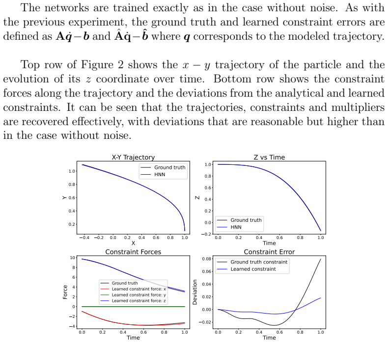
Adding 2% multiplicative noise to the training data increases trajectory divergence over long horizons but keeps normalized constraint-force errors low, around 1-2%, suggesting that the learned constraint structure is relatively robust to imperfect data.
The architecture is not restricted to holonomic constraints; it treats any linear constraint of the form $A \dot q = b$, integrable or not.
If the learned Hamiltonian and constraints are correct, the network can be used to predict energy and constraint forces for applications such as noise prediction, dissipation detection, and robot control.

Reading between the lines

Editorial extensions of the paper, not claims the author makes directly.

Because the loss only pins down the combined term $\partial H/\partial q - A^T \lambda$, any practical deployment should validate learned constraint forces against an analytical force law before relying on them for control; the paper's uniqueness analysis covers only a fixed constraint matrix $A$.
The same architecture could serve as a data-driven way to discover nonholonomic constraint equations from raw robot trajectories, since the constraint network directly outputs a matrix $A(q)$ and vector $b(q)$ that can be read off after training.
For systems where measurements provide positions and velocities but not momenta, the method could be chained to a learned momentum map, though the paper lists such extensions as future work.
Because gauge transformations such as rescaling or linearly combining constraints leave the dynamics invariant, learned representations of $A$ and $\lambda$ may differ between runs; quantifying this gauge freedom would tell users how much of the learned structure is physical.

Share X Bluesky LinkedIn Reddit HN

Signed reviews

No signed human review yet.

Editorial analysis

A structured set of objections, weighed in public.

Desk editor's note, referee report, and a circularity audit.

Desk Editor's Note

read the letter

Plainly: the paper is a worthwhile architecture paper, but its central claim—that it simultaneously recovers the Hamiltonian, constraints, and Lagrange multipliers—outruns the evidence. The identifiability problem is real, and the supplement does not close it.

What's new: unlike Altawaitan et al., which assumes the constraints are known, this three-network setup learns A, b, and λ from data. The loss is a direct encoding of the pseudo-Hamiltonian equations plus the constraint residual, and the architecture is straightforward. The experiments are internally consistent: rolling disk, solid and hollow sphere on a spinning table, and a point mass in the supplement, each with and without noise. The authors even ask the right question about whether the networks learn the intended quantities and provide a supplementary proof attempt. That is honest and useful.

The soft spot is the identifiability of the decomposition. The loss only constrains ∂H/∂q − A^T λ and A q̇ − b. The gauge freedoms in Eqs. 5–6 are acknowledged, but the supplement fixes A and then checks the curl condition (Eq. 9) only for the 3D point mass. The rolling disk and spinning table matrices are never subjected to Eq. 9. Worse, there is an exact symmetry the paper misses: for a holonomic constraint g(q)=0 with A=∂g/∂q, any smooth F gives H'=H+F(g), λ'=λ+F'(g), and the loss is unchanged identically. Since the paper explicitly includes holonomic constraints, the slogan about simultaneously learning H and λ is false in that case. For nonholonomic systems the analogous mixing can occur if the constraint annihilator contains an exact one-form; the paper gives no reason it does not. So the experiments show trajectory and constraint fitting, not uniquely identified physics.

Minor but worth noting: no baselines, no repeated-seed error bars, no released code or data. Those could be fixed in revision. The 229-hour training time on one disk trajectory is also worth scrutiny, though not a flaw by itself.

Who should read it: people building HNN variants and anyone looking for a cautionary tale about identifiability in physics-informed learning. The architecture is a reasonable contribution, but the claims need to be reined in or proven. I'd send it to peer review—a serious referee can sort out the identifiability question—but I would not cite it as evidence of simultaneous physical recovery until that is resolved.

Referee Report

3 major / 6 minor

Summary. The paper proposes a three-network Hamiltonian-based architecture for learning the dynamics of constrained mechanical systems from phase-space data. One network learns the Hamiltonian H(q,p), a second learns the constraint matrix A(q) and vector b(q), and a third learns the Lagrange multiplier vector λ(q,p). The networks are trained with the single loss in Eq. (7), which enforces the constrained Hamilton equations and the linear constraint A qdot − b = 0. The method is tested on a rolling disk and on solid and hollow balls on a spinning table, with and without 2% multiplicative noise, and a supplementary experiment on a 3D nonholonomically constrained particle is included. Reported results include trajectory predictions, constraint residuals, mean-shifted energy MAE, normalized constraint-force error, and Lyapunov divergence times. The supplementary material also contains a proof intended to establish uniqueness of H and λ for a fixed constraint matrix A.

Significance. If the central identifiability claim were established, the paper would make a useful contribution to data-driven nonholonomic mechanics: recovering H, A, b, and λ simultaneously from unlabelled phase-space data would enable energy and constraint-force estimation in robotics and control. The paper is clearly written, the architecture and training loss are fully specified, and the trajectory predictions in Figs. 3, 5, and 6 are accurate with small constraint residuals, both clean and noisy. The supplementary uniqueness attempt is a genuinely constructive step beyond purely empirical benchmarking. However, as detailed below, the identifiability proof covers only one toy example, an exact symmetry invalidates the claim for the stated holonomic scope, and the ball-on-table experiments omit a necessary holonomic constraint on the Euler-Rodrigues parameters. The paper therefore currently demonstrates trajectory and constraint-residual fitting rather than the certified recovery of H and λ.

major comments (3)

[Supplementary §2; main §2.2, Eq. (7)] The uniqueness proof is not sufficient to support the claim that H, A, b, and λ are simultaneously learned. The proof is carried out only for the point-mass constraint matrix A = [−y, 0, 1], and the rolling-disk and spinning-table matrices (Eqs. 10 and 15) are never checked against condition Eq. (9). Moreover, the proof fixes A, whereas in training A is a learned quantity. Because the loss Eq. (7) constrains only the combined term ∂H/∂q − A^T λ and the residual A qdot − b, any alternative decomposition that leaves these two combinations unchanged is invisible to the training objective. Please either prove that no nonzero λ* satisfies ∇ × (A^T λ*) = 0 for each experimental constraint matrix, including the gauge transformations of Eqs. (5)–(6), or explicitly introduce an identifiability assumption/regularization and state the resulting scope of the claim.
[§2.1, §2.2, Eq. (7)] The stated scope includes holonomic constraints, and there the central claim is exactly false. For a holonomic constraint g(q) = 0 with A = ∂g/∂q in the time-differentiated form, any smooth F gives H' = H + F(g) and λ' = λ + F'(g), and one verifies that ∂H'/∂p = ∂H/∂p, ∂H'/∂q − A^T λ' = ∂H/∂q − A^T λ, and A qdot − b = dg/dt = 0, so the loss Eq. (7) is unchanged exactly. Thus infinitely many (H, λ) pairs with different reported energies and constraint forces fit the training objective identically, and the mean-shifted energy MAE in Tables 5–6 cannot distinguish them. The authors should either narrow the claim to the nonholonomic setting or add a mechanism that breaks this symmetry, such as an additional energy-conservation residual or auxiliary information about H.
[§3.2, Eqs. (13)–(15)] The ball-on-spinning-table experiments omit the holonomic unit-norm constraint on the Euler-Rodrigues parameters. The Hamiltonian in Eq. (13) and the momenta in Eq. (14) are only valid on the unit sphere ||e||^2 = 1, and with e_dot = p_e/(4I) the unconstrained flow leaves that sphere unless the additional velocity constraint e · e_dot = 0 is imposed. The learned A network outputs only two constraint rows, those in Eq. (15), so the architecture has no explicit mechanism to preserve ||e|| = 1. Please include the quaternion normalization as an additional constraint row (or justify that it is automatically satisfied), and report the e-norm error along the learned trajectories, particularly in the noisy experiments.

minor comments (6)

[§3.1, Table 1] The learning-rate entry for the λ and A networks is marked with an asterisk, but the table has no footnote; the text mentions reductions at 1.5e5 and 3e5 epochs, so the table should state the schedule explicitly.
[Throughout] The word 'asses' is used repeatedly where 'assess' is intended; please run a spelling pass over the manuscript.
[Reference [11]] The in-text citation appears as 'Alltawaitan et al.' while the reference list spells the first author 'Altawaitan'; please unify the spelling.
[§3.4] The Lyapunov-exponent calculation is described only briefly: initial 30% of the error vector is removed and the remainder is normalized, but the fitting window and the number of trajectories used are not stated. Please specify these details for reproducibility.
[§3.1, Eq. (11)] The expression for phi_dot is ambiguous because the parentheses are unbalanced in the printed form; please rewrite it with unambiguous notation.
[General] No statement of code or data availability is included; providing the trained-model code would improve reproducibility and allow readers to test the identifiability issue directly.

Circularity Check

0 steps flagged · score 0.0 of 10

No significant circularity: the loss is an inverse-problem residual and all learned quantities are benchmarked against independently defined ground-truth functions.

full rationale

The proposed method does not derive H, A, b, or λ from the loss by definition; it trains three networks to minimize the residual of Eqs. (2)-(3), which are standard mechanical equations taken from the literature, and then checks the learned functions against analytical Hamiltonians (Eqs. 8 and 13), analytical constraints (Eqs. 10 and 15), and ground-truth trajectories generated from the same equations. This is a physics-prior inverse problem, not a tautology: the true H, A, λ are never used as labels, and a network could in principle fit the residuals without matching them, which is why the supplementary material attempts a uniqueness proof. That proof is an independent mathematical argument (differences of solutions reduce to ∂H*/∂q = A^T λ* and the curl condition), not a restatement of the loss. The paper contains no load-bearing self-citations: the cited pseudo-Hamiltonian formulation [18]-[20] is external prior work. The identifiability gap noted in the supplement (Eq. 9 is verified only for the point-mass A, not for the rolling-disk or spinning-table A, and holonomic constraints admit exact loss-invariant transformations H→H+F(g), λ→λ+F'(g)) is a correctness and generalization concern, not circularity; it does not make the reported trajectory or energy benchmarks coincide with the training objective by construction.

Assumptions & free parameters 3 free parameters · 5 assumptions · 0 invented entities

The central method rests on standard constrained Hamilton equations and the assumption that constraints are linear in velocities. The benchmark uses synthetic data from textbook analytical models. Network hyperparameters and an energy-offset normalization are chosen by hand. No new physical entities are introduced.

free parameters (3)

Learning-rate schedule for A and λ networks (rolling disk) = 5e-5, reduced to 2e-5 after 1.5e5 epochs, then 1e-5 after 3e5 epochs
Reported in Table 1; the schedule was chosen empirically to facilitate convergence, so the reported results depend on this tuning.
Energy comparison offset = mean of predicted energy shifted to mean of ground truth
Used in Section 3.4 before computing MAE; justified because H is unique up to a constant, but it is a hand-chosen normalization.
Network size hyperparameters = H/A/λ hidden neurons: 200/400/300 for disk, 200/50/200 for ball
Chosen by hand in Tables 1 and 3; no sensitivity analysis is provided.

assumptions (5)

domain assumption The constrained Hamilton equations ˙q = ∂H/∂p and ˙p = -∂H/∂q + A^T λ hold for the systems considered.
Used to build the loss in Eq 7; standard result from the pseudo-Hamiltonian formulation [18].
domain assumption Constraints can be written as linear in velocities, A(q) ˙q = b(q), with A and b independent of ˙q.
Eq 2; this excludes general nonlinear nonholonomic constraints except by local linear approximation.
domain assumption A is smooth enough that differentiating A ˙q = b yields λ as a function of q and p.
Section 2.1, Eq 4 requires differentiating the constraint equation to solve for λ.
ad hoc to paper The multilayer perceptrons can represent H, A, b, and λ accurately enough, and gradient descent converges to a good minimum.
Implicit in all experiments; not proven, and no seed variability is reported.
domain assumption Synthetic data generated from known analytical models are representative of real measurements.
All experiments use simulated data; no experimental measurements are used.

how reviews work

0 comments

Cite this review

Pith. "Pith review of Hamiltonian-based neural networks for systems under nonholonomic constraints." pith.science (2026). https://pith.science/paper/3KAXLO65

@misc{pith2026241203018,
  author       = {Pith},
  title        = {Pith review of: Hamiltonian-based neural networks for systems under nonholonomic constraints},
  year         = {2026},
  howpublished = {\url{https://pith.science/paper/3KAXLO65}},
  note         = {Machine review of arXiv:2412.03018}
}

read the original abstract

There has been increasing interest in methodologies that incorporate physics priors into neural network architectures to enhance their modeling capabilities. A family of these methodologies that has gained traction are Hamiltonian neural networks (HNN) and their variations. These architectures explicitly encode Hamiltonian mechanics both in their structure and loss function. Although Hamiltonian systems under nonholonomic constraints are in general not Hamiltonian, it is possible to formulate them in pseudo-Hamiltonian form, equipped with a Lie bracket which is almost Poisson. This opens the possibility of using some principles of HNNs in systems under nonholonomic constraints. The goal of the present work is to develop a modified Hamiltonian neural network architecture capable of modeling Hamiltonian systems under holonomic and nonholonomic constraints. A three-network parallel architecture is proposed to simultaneously learn the Hamiltonian of the system, the constraints, and their associated multipliers. A rolling disk and a ball on a spinning table are considered as canonical examples to assess the performance of the proposed Hamiltonian architecture. The experiments are then repeated with a noisy training set to study modeling performance under more realistic conditions.

Figures

Figures reproduced from arXiv: 2412.03018 by the authors.

**Figure 2.** a) The coordinates x and y indicate the position of the point of contact between the disk and the surface, ϕ represents the rolling angle of the disk about its symmetry axis, and ψ is the angle of rotation with respect to the vertical axis. b) θ is the leaning angle of the disk from its fully vertical position. The Hamiltonian of the system is H = p 2 x + p 2 y 2m + p 2 ϕ 2Ixx + (pψ + pϕ sin(θ))2 cos2 (θ)Ixx + p 2 θ… view at source ↗

**Figure 3.** Trajectories and deviations for the rolling disk system. [PITH_FULL_IMAGE:figures/full_fig_p013_3.png] view at source ↗

Figures from the paper (11 more)

**Figure 4.** Figure 4: The position of the ball with respect to the center of the table is given by the [PITH_FULL_IMAGE:figures/full_fig_p015_4.png]

**Figure 5.** Figure 5: Trajectories and deviations for the solid ball on spinning table. [PITH_FULL_IMAGE:figures/full_fig_p017_5.png]

**Figure 6.** Figure 6: Trajectories and deviations for the hollow ball on spinning table. [PITH_FULL_IMAGE:figures/full_fig_p017_6.png]

**Figure 7.** Figure 7: Trajectories and deviations for the rolling disk system in the presence of noise. [PITH_FULL_IMAGE:figures/full_fig_p019_7.png]

**Figure 8.** Figure 8: Trajectories and deviations for the solid ball on spinning table with noise. [PITH_FULL_IMAGE:figures/full_fig_p020_8.png]

**Figure 9.** Figure 9: Results for the hollow ball on spinning table with noise. [PITH_FULL_IMAGE:figures/full_fig_p020_9.png]

**Figure 10.** Figure 10: Evolution of the training and validation loss functions for the experiments [PITH_FULL_IMAGE:figures/full_fig_p023_10.png]

**Figure 11.** Figure 11: Evolution of the training and validation loss functions for the experiments with [PITH_FULL_IMAGE:figures/full_fig_p023_11.png]

**Figure 1.** Figure 1: Trajectories and deviations for the nonholonomically constrained particle . [PITH_FULL_IMAGE:figures/full_fig_p030_1.png]

**Figure 2.** Figure 2: Trajectories and deviations for the point mass system in the presence of noise. [PITH_FULL_IMAGE:figures/full_fig_p031_2.png]

**Figure 3.** Figure 3: Evolution of the training and validation loss functions for the nonholonomically [PITH_FULL_IMAGE:figures/full_fig_p032_3.png]

Discussion (0). Continue with ORCID to comment.

Reference graph

Works this paper leans on

28 extracted references · 23 canonical work pages

[1]

Conti, G

P. Conti, G. Gobat, S. Fresca, A. Manzoni, A. Frangi, Reduced or- der modeling of parametrized systems through autoencoders and sindy approach: continuation of periodic solutions, Computer Methods in Ap- plied Mechanics and Engineering 411 (2023) 116072

work page 2023
[2]

Hansen, X

C. Hansen, X. I. Yang, M. Abkar, Data-driven dynamical system models of roughness-induced secondary flows in thermally stratified turbulent boundary layers, Journal of Fluids Engineering 145 (6) (2023) 061102

work page 2023
[3]

K. Lee, N. Trask, P. Stinis, Structure-preserving sparse identification of nonlinear dynamics for data-driven modeling, in: Mathematical and Scientific Machine Learning, PMLR, 2022, pp. 65–80

work page 2022
[4]

P. J. Schmid, Dynamic mode decomposition of numerical and experi- mental data, Journal of fluid mechanics 656 (2010) 5–28

2010
[5]

Andreuzzi, N

F. Andreuzzi, N. Demo, G. Rozza, A dynamic mode decomposition extension for the forecasting of parametric dynamical systems, SIAM Journal on Applied Dynamical Systems 22 (3) (2023) 2432–2458

2023
[6]

Morandin, J

R. Morandin, J. Nicodemus, B. Unger, Port-hamiltonian dynamic mode decomposition, SIAM Journal on Scientific Computing 45 (4) (2023) A1690–A1710

work page 2023
[7]

T. W. Cornforth, H. Lipson, A hybrid evolutionary algorithm for the symbolic modeling of multiple-time-scale dynamical systems, Evolution- ary Intelligence 8 (2015) 149–164

work page 2015
[8]

Raissi, P

M. Raissi, P. Perdikaris, G. E. Karniadakis, Physics-informed neural networks: A deep learning framework for solving forward and inverse 24 problems involving nonlinear partial differential equations, Journal of Computational physics 378 (2019) 686–707

work page 2019

Show all 28 references

[9]

Greydanus, M

S. Greydanus, M. Dzamba, J. Yosinski, Hamiltonian neural networks, Advances in neural information processing systems 32 (2019)

2019
[10]

Course, T

K. Course, T. Evans, P. Nair, Weak form generalized hamiltonian learn- ing, Advances in Neural Information Processing Systems 33 (2020) 18716–18726

2020
[11]

Altawaitan, J

A. Altawaitan, J. Stanley, S. Ghosal, T. Duong, N. Atanasov, Hamilto- nian dynamics learning from point cloud observations for nonholonomic mobile robot control, arXiv preprint arXiv:2309.09163 (2023)

2023 arXiv
[12]

Weinan, et al., The dawning of a new era in applied mathematics, Notices of the American Mathematical Society 68 (4) (2021) 565–571

E. Weinan, et al., The dawning of a new era in applied mathematics, Notices of the American Mathematical Society 68 (4) (2021) 565–571

2021
[13]

Nakamura-Zimmerer, Q

T. Nakamura-Zimmerer, Q. Gong, W. Kang, Adaptive deep learning for high-dimensional hamilton–jacobi–bellman equations, SIAM Journal on Scientific Computing 43 (2) (2021) A1221–A1247

2021
[14]

Sosanya, S

A. Sosanya, S. Greydanus, Dissipative hamiltonian neural networks: Learning dissipative and conservative dynamics separately, arXiv preprint arXiv:2201.10085 (2022)

2022 arXiv
[15]

S. A. Desai, M. Mattheakis, D. Sondak, P. Protopapas, S. J. Roberts, Port-hamiltonian neural networks for learning explicit time-dependent dynamical systems, Physical Review E 104 (3) (2021) 034312

2021
[16]

Sarasola, F

C. Sarasola, F. Torrealdea, A. d’Anjou, A. Moujahid, M. Gra˜ na, Energy balance in feedback synchronization of chaotic systems, Physical Review E 69 (1) (2004) 011606

2004
[17]

C.-D. Han, B. Glaz, M. Haile, Y.-C. Lai, Adaptable hamiltonian neural networks, Physical Review Research 3 (2) (2021) 023156

2021
[18]

Van der Schaft, B

A. Van der Schaft, B. Maschke, On the hamiltonian formulation of non- holonomic mechanical systems, Reports on mathematical physics 34 (2) (1994) 225–233. 25

1994
[19]

de Le´ on, M

M. de Le´ on, M. Lainz, A. L´ opez-Gord´ on, J. C. Marrero, Nonholonomic brackets: Eden revisited, in: International Conference on Geometric Science of Information, Springer, 2023, pp. 105–112

2023
[20]

Eden, The hamiltonian dynamics of non-holonomic systems, Pro- ceedings of the Royal Society of London

R. Eden, The hamiltonian dynamics of non-holonomic systems, Pro- ceedings of the Royal Society of London. Series A. Mathematical and Physical Sciences 205 (1083) (1951) 564–583

1951
[21]

Duong, N

T. Duong, N. Atanasov, Hamiltonian-based neural ode networks on the se (3) manifold for dynamics learning and control, arXiv preprint arXiv:2106.12782 (2021)

2021 arXiv
[22]

Goldstein, Classical mechanics, Pearson Education India, 2011

H. Goldstein, Classical mechanics, Pearson Education India, 2011

2011
[23]

Rosenberg, Analytical dynamics, Springer, 1977

R. Rosenberg, Analytical dynamics, Springer, 1977

1977
[24]

Bloch, et al., Nonholonomic mechanics and control [electronic re- source]

A. Bloch, et al., Nonholonomic mechanics and control [electronic re- source]
[25]

Wittenburg, Dynamics of multibody systems, Springer, 1980

J. Wittenburg, Dynamics of multibody systems, Springer, 1980. 26 Hamiltonian-based neural networks for systems under nonholonomic constraints: Supplementary material Ignacio Puiggros T. a, A. Srikantha Phani a aDepartment of Mechanical Engineering, The University of British Co...

1980
[26]

Nonholonomically constrained particle 1.1. System description As a proof of concept, we choose a simple system consisting of a particle moving in three dimensions under the effect of gravity and under a single nonholonomic constraint. The Hamiltonian of the system is H = (p2 x...

2024 arXiv
[27]

Both the learned and ground truth constraints deviations are close to zero, with the former being lower

It can be seen that both the trajectory and the constraint forces match the ground truth with high precision. Both the learned and ground truth constraints deviations are close to zero, with the former being lower. This 2 is probably due to the fact that the loss function in e...
[28]

Uniqueness of ˆH and ˆλ A relevant question is whether the three networks will learn exactly and only the quantity they are assigned to. In principle, the networks could learn in such a way that both ˙q and ˙p are properly modeled, but the terms ˆH and ˆA T ˆλ do not correspon...

Pith tools

Reviewed August 11, 2026 · model on record in the stance chip above.

[1] [1]

Conti, G

P. Conti, G. Gobat, S. Fresca, A. Manzoni, A. Frangi, Reduced or- der modeling of parametrized systems through autoencoders and sindy approach: continuation of periodic solutions, Computer Methods in Ap- plied Mechanics and Engineering 411 (2023) 116072

work page 2023

[2] [2]

Hansen, X

C. Hansen, X. I. Yang, M. Abkar, Data-driven dynamical system models of roughness-induced secondary flows in thermally stratified turbulent boundary layers, Journal of Fluids Engineering 145 (6) (2023) 061102

work page 2023

[3] [3]

K. Lee, N. Trask, P. Stinis, Structure-preserving sparse identification of nonlinear dynamics for data-driven modeling, in: Mathematical and Scientific Machine Learning, PMLR, 2022, pp. 65–80

work page 2022

[4] [4]

P. J. Schmid, Dynamic mode decomposition of numerical and experi- mental data, Journal of fluid mechanics 656 (2010) 5–28

2010

[5] [5]

Andreuzzi, N

F. Andreuzzi, N. Demo, G. Rozza, A dynamic mode decomposition extension for the forecasting of parametric dynamical systems, SIAM Journal on Applied Dynamical Systems 22 (3) (2023) 2432–2458

2023

[6] [6]

Morandin, J

R. Morandin, J. Nicodemus, B. Unger, Port-hamiltonian dynamic mode decomposition, SIAM Journal on Scientific Computing 45 (4) (2023) A1690–A1710

work page 2023

[7] [7]

T. W. Cornforth, H. Lipson, A hybrid evolutionary algorithm for the symbolic modeling of multiple-time-scale dynamical systems, Evolution- ary Intelligence 8 (2015) 149–164

work page 2015

[8] [8]

Raissi, P

M. Raissi, P. Perdikaris, G. E. Karniadakis, Physics-informed neural networks: A deep learning framework for solving forward and inverse 24 problems involving nonlinear partial differential equations, Journal of Computational physics 378 (2019) 686–707

work page 2019