Solving Self-calibration of ALMA Data with an Optimization Method

Masayuki Yamaguchi; Shiro Ikeda; Takashi Tsukagoshi; Takeshi Nakazato; Tsutomu T. Takeuchi

REVIEW 3 major objections 4 minor 32 references

Solving Self-calibration of ALMA Data with an Optimization Method

T0 review · 3 major / 4 minor · reviewed 2026-08-11 · deepseek-v4-flash

Challenge this review Re-run · record.json Download PDF Read on arXiv ↗ Review JSON

Pith's one-line read This paper turns the gain-correction step of radio-interferometry self-calibration into a regularized optimization problem and, combined with its RML imaging method, reformulates the entire self-calibration loop as a single optimization…

desk verdict Well-built joint self-calibration/imaging framework, but the empirical case rests on hand-set gain variance targets and no baseline comparison; still deserves serious refereeing. read the letter →

arxiv 2412.03183 v1 pith:QLNLQJEA submitted 2024-12-04 astro-ph.IM stat.AP

Shiro Ikeda , Takeshi Nakazato , Takashi Tsukagoshi , Tsutomu T. Takeuchi , Masayuki Yamaguchi This is my paper · ORCID

classification astro-ph.IMstat.AP

keywords self-calibrationradiointerferometryALMAgaincorrectionregularizedmaximumlikelihoodsparsemodelingtotalsquaredvariationBayesianoptimization

verification ladder T0 review T1 audit T2 compute T3 formal

The pith

A machine-rendered reading of the paper's core claim, the machinery that carries it, and where it could break.

The reading

Radio interferometry images are corrupted by time-varying per-antenna gains, and the standard fix, self-calibration, alternates between CLEAN imaging and manual gain adjustment. This paper argues that both jobs can instead be written as one objective: a data-fidelity term plus sparsity and smoothness regularization on the image plus a temporal-smoothness penalty on the gains, all minimized alternately. On three ALMA data sets the corrected images are sharper and have higher peak intensity than the same imaging method without self-calibration, while the estimated gains vary smoothly in time as atmospheric fluctuations would. The cost is that the amount of allowed gain variation is set by hand-picked target variances; the paper leaves an objective choice of those targets to future work.

What carries the argument

The load-bearing object is the combined regularized objective of equation (14). Its gain term $S_{\mu_1,\mu_2}(g)$ is what turns self-calibration into optimization: it pulls adjacent-in-time gains toward one another through weights $w_{\alpha l}=1/(t_l-t_{l-1})$, with $\mu_1$ penalizing changes in the complex gain and $\mu_2$ penalizing only amplitude changes, while the normalization constraint prevents all gains from collapsing to zero. Because the joint objective is non-convex, the algorithm alternates a convex image step (PRIISM with $\ell^1$ plus total squared variation, solved by MFISTA using a non-uniform FFT) and a gain step solved by the duplicate-variable quadratic surrogate in Appendix 1, whose closed-form update is refined by increasing the coupling parameter $\rho$. The four regularization weights are chosen by alternating Bayesian optimization: the image weights are selected so the reconstructed image's power lies inside the covering u-v ellipsoid and the visibility residuals are uniform over u-v distance, while the gain weights are selected to bring the phase and amplitude standard deviations $(\sigma_{\rm ph},\sigma_{\rm amp})$ to hand-set targets $(\sigma^*_{\rm ph},\sigma^*_{\rm amp})$.

What would settle it

Simulate an ALMA-like observation with a known sky image and known time-varying antenna gains, run the proposed method with the paper's hand-set variance targets, and compare the recovered gains and image with the truth: the central claim fails if the recovered image is no better than the one with gains fixed to unity, or if the ranking of the two hand-set target choices reverses the reported sharpening.

Watch

Extended reading notes

Core claim

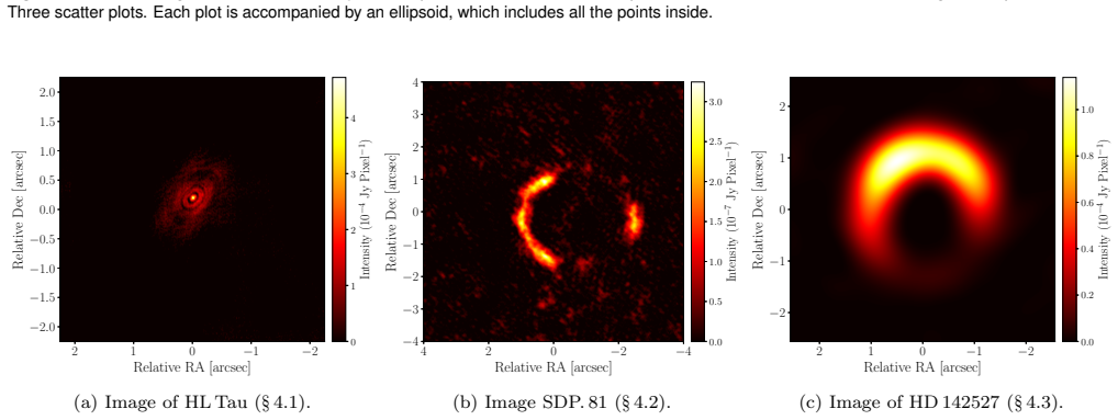
The paper's central claim is that self-calibration can be reduced to the joint minimization of equation (14), $L_{\tilde v}(x,g) + R_{\lambda_1,\lambda_2}(x) + S_{\mu_1,\mu_2}(g)$, over an image $x\ge 0$ and complex antenna gains $g$ with $\sum_l |g_{\alpha l}|=N_\alpha$. Here $L_{\tilde v}$ is the weighted visibility likelihood, $R$ combines the $\ell^1$ norm and total squared variation to favor sparse, smooth images, and $S$ penalizes squared time differences of the complex gains and of their amplitudes. The joint problem is non-convex, so the paper solves it by alternating the PRIISM image update and a gain update obtained from a quadratic surrogate that has the closed-form solution $\hat g_{\alpha l}=r_{\alpha l} b_{\alpha l}/|b_{\alpha l}|$ from Appendix 1. The authors report that on HL Tau, SDP.81, and HD 142527 the reconstructed images appear sharper with higher peak intensities than without self-calibration, and the estimated gains change smoothly in time.

Load-bearing premise

The whole procedure leans on the hand-set target gain variances $(\sigma^*_{\rm ph},\sigma^*_{\rm amp})$ that pick the regularization strengths $\mu_1,\mu_2$; the paper sets these targets by hand and says an objective way to derive them from ALMA data is future work.

Editorial extensions

If this is right

The traditional hand-tuned loop of CLEAN plus separate gain solutions is replaceable by alternating a convex image update and a closed-form gain update within one objective.
The temporal-smoothness penalties on gains encode the physical expectation that atmospheric phase and amplitude errors evolve continuously, so estimated gains become smooth time series rather than piecewise constant solution intervals.
On all three data sets the method produces sharper images and higher peak intensities than no self-calibration, with the degree of correction controlled by the target gain variances.
Because the formulation separates the objective from the solver, other image regularizers or gain priors can be dropped into equation (14) without redesigning the self-calibration logic.
The announced public release of the self-calibration module alongside PRIISM would let ALMA users apply RML self-calibration without building their own gain solvers.

Reading between the lines

Editorial extensions of the paper, not claims the author makes directly.

A natural next step is an objective, data-driven rule for the target gain variances; linking them to weather diagnostics such as phase-monitor RMS or precipitable-water-vapor measurements would test whether the hand-set values are replaceable.
A direct head-to-head comparison with CLEAN-based self-calibration on identical data would separate how much of the sharpening comes from the gain correction and how much from the RML image prior.
The same alternating scheme could extend to polarization, multiband, and spectral-line imaging, since those enter only through the data-fidelity term and the regularizers.

Share X Bluesky LinkedIn Reddit HN

Signed reviews

No signed human review yet.

Editorial analysis

A structured set of objections, weighed in public.

Desk editor's note, referee report, and a circularity audit.

Desk Editor's Note

read the letter

The core of this paper is a reformulation of ALMA self-calibration as a single regularized optimization problem, alternating PRIISM imaging with a smoothness-regularized gain update. That specific combination is genuinely new and worth engaging with. The derivation is coherent, the closed-form gain update in Appendix 1 is re-implementable, and the time-smoothness regularizers are a sensible way to encode the expected behavior of atmospheric gain fluctuations. The Bayesian parameter search over the four hyperparameters is pragmatic and clearly described. The authors also deserve credit for testing on three real ALMA data sets rather than simulated data alone.

The soft spots are real and mostly in the evaluation. The main one: section 3.4 selects μ1 and μ2 by minimizing Eq. (17), which explicitly forces the estimated gain scatter (σph, σamp) toward target values (σ*_ph, σ*_amp) that are set by hand. The paper says so plainly and defers an objective choice to future work. Because the gains are never observed, the tables reporting achieved σph and σamp are therefore outputs of the fitting procedure, not independent validation. The "sharper images and higher peaks" under the Large variance targets are a direct consequence of asking for larger gain variance, not evidence that the gains are correctly estimated. This is a load-bearing issue for the claim of "promising results." A second issue is that C1 and C2 are used both to select λ and then reported as quality metrics; that is circular, though the constraints are soft and the measures may still be useful for avoiding overfitting. Third, there is no comparison with standard CLEAN-based self-calibration, no injected gain errors, and no quantified baseline. The paper explicitly acknowledges this as ongoing work, which is honest but leaves the central empirical claim unestablished.

None of this undercuts the mathematical formulation itself. The method is well posed, the algorithm is specified in enough detail to re-implement, and the questions raised are addressable with additional experiments. The lack of released code for the self-calibration part is a practical inconvenience but not a scientific flaw.

This paper is for ALMA users and RML practitioners looking for a principled alternative to the hand-tuned CLEAN/self-calibration loop. It deserves serious refereeing, but the referee should push for a baseline comparison and either an objective way to set the gain variance targets or a sensitivity analysis showing that the results are robust to them.

Referee Report

3 major / 4 minor

Summary. The paper reformulates radio-interferometric self-calibration as a joint regularized optimization over the image and per-antenna time-dependent complex gains (Eq. 14). The image subproblem is solved with the authors' PRIISM RML method (Eq. 10), and the gain subproblem is solved with a closed-form update derived through variable splitting (Appendix 1, Eqs. A1–A5). The four regularization parameters are selected by Bayesian optimization using two image-domain criteria C1 and C2 (Eq. 16) and gain variance targets (Eq. 17). The method is demonstrated on three ALMA data sets (HL Tau, SDP.81, HD 142527), each with 'small' and 'large' hand-set gain variance targets. The reported results are qualitative: reconstructed images are described as sharper with higher peak intensity than without self-calibration, the estimated gains vary smoothly in time, and achieved values of C1, C2, sigma_ph, and sigma_amp are tabulated.

Significance. If the gain estimates are correct, the formulation offers a principled, modular alternative to the iterative CLEAN/self-calibration loop, extending the RML framework to gain calibration with tunable temporal regularization. The closed-form gain update is a useful contribution, and testing on three real ALMA data sets of different morphologies is a strength. However, the current evaluation is self-referential: the same statistics used to select parameters are then reported as validation, and no comparison with standard CLEAN-based self-calibration or with injected gain errors is made. The significance therefore hinges on future validation; as it stands, the claim of 'promising results' is plausible but not yet established.

major comments (3)

[§3.4, Eq. (16); Tables 2, 4, 6] The selection of lambda_1 and lambda_2 minimizes Eq. (16), which contains penalties hsq(C1* - C1) + hsq(C2* - C2) with C1* = 0.995 and C2* = 0.99, and the selection of mu_1 and mu_2 minimizes Eq. (17), which drives sigma_ph and sigma_amp toward hand-set targets. The paper then reports the achieved C1, C2, sigma_ph, and sigma_amp in Tables 2, 4, and 6 as evidence of image and gain quality. This is circular: these quantities are optimized to satisfy those conditions, so they cannot independently validate the reconstruction. The text should either present C1 and C2 only as enforced constraints, or provide independent validation metrics.
[§4.1, Figs. 3–5; §5] The empirical evidence for improvement is limited to qualitative statements that the images 'give sharper impressions' and have higher peak intensities than the no-self-calibration case. Because larger allowed gain variance directly permits larger gain fluctuations, the fact that the 'Large variance' runs produce sharper, higher-peak images is a direct consequence of the hand-set targets rather than evidence that the estimated gains are correct. The absence of a comparison with standard CLEAN-based self-calibration or with simulated data with known injected gain errors—both deferred to future work in §5—means the central claim of 'promising results' is not yet supported by the experiments as presented.
[§3.4, Eq. (17); §5] The target gain variances sigma*_ph and sigma*_amp are set by hand ('We set the target values by hand in this work'), and the paper states that an objective choice from ALMA observations is future work. Since the true gains are unknown, the output of the method depends on these free parameters. The paper needs either a principled, data-driven procedure for setting the targets, or a demonstration that the reconstructions are insensitive to reasonable target choices. The two hand-picked cases shown are not sufficient to establish robustness.

minor comments (4)

[§4.1] The sentence 'The gains of figures 3b, have larger variances than those of figures 3e' contradicts the figure labels; the Small-variance gains in Fig. 3b should have smaller variances than the Large-variance gains in Fig. 3e.
[Appendix 1, Eq. (A5)] The symbol y_k in the definition of b_{alpha l} is not defined in the manuscript; it should be introduced explicitly (presumably the model visibility F_k(x) or the calibrated visibility).
[§3.4] The search over lambda_1, lambda_2, mu_1, and mu_2 is restricted to integer values of their logarithms and limited to 30 Bayesian optimization trials, but the search ranges for Lambda_1, Lambda_2, M_1, and M_2 are not stated; because some selected values lie at the edge of the reported tables (e.g., Lambda_2 = 13 in Table 5), it is unclear whether the optimum is inside the allowed grid.
[Table 6] For HD 142527 with Small variance, C2 = 0.845, which is far below the C2 >= 0.99 target used in Eq. (16); the text acknowledges this, but it should be discussed explicitly as a failure of the parameter-selection loop to satisfy its own constraint, and the implications for the reconstructed image should be addressed.

Circularity Check

2 steps flagged · score 6.0 of 10

The reported validation is partly circular: λ selection enforces the C1/C2 thresholds that are then presented as quality metrics, and gain scatters in the tables are fitted to hand-set targets by Eq. (17).

fitted input called prediction [Section 3.4, Eq. (16); Section 4, Tables 2/4/6 and §4.1 text]
"For {λ1, λ2}, the Bayesian optimization problem is defined as min_{λ1,λ2} [ L ˜v( ˆx, ˆg) + κ ( hsq(C ∗ 1 − C1) + hsq(C ∗ 2 − C2) ) ] ... and we set κ = 10^6 in § 4. ... The statistics related to the image and the gains are shown in table 2. Almost all the power of the image is concentrated in the covering ellipsoid (C1 > 0.99), and the power of the residual is distributed equally over u–v distance (C2 > 0.99)."

C1 and C2 are not independent diagnostics: they are the exact quantities appearing in the soft constraints of Eq. (16), with a huge penalty κ = 10^6 driving the selected λ1, λ2 toward C1 ≥ 0.995 and C2 ≥ 0.99. Reporting the resulting C1, C2 values in Tables 2, 4, 6 and reading the threshold satisfaction as evidence of a good image-model fit is therefore reporting the objective's own penalty terms. The 'almost all power...' statements in §4 restate the selection constraints rather than validate the reconstruction from the data.
fitted input called prediction [Section 3.4, Eq. (17); Section 4, Tables 2/4/6; Conclusion]
"The parameters µ1 and µ2 are chosen to make (σph, σamp) close to a given target values (σ∗ ph, σ∗ amp). We set the target values by hand in this work. ... Since we do not know the true gains, how to define the variances of gains from ALMA observation information is an open problem."

Eq. (17) explicitly minimizes the relative distance of the estimated gain scatters (σph, σamp) to hand-set targets. Hence the σph and σamp values in Tables 2, 4, 6 (e.g. 4.68 deg vs 16.9 deg for HL Tau) are produced to match the 'Small variance' and 'Large variance' inputs, not inferred from data. The paper's observation that larger targets give sharper images with higher peak intensities is the expected consequence of allowing larger gain modulation, as the paper itself states in §3.4, and cannot validate the gain correction without ground-truth gains or a comparison to CLEAN-based self-calibration. The Conclusion concedes this selection principle is open and the CLEAN comparison is ongoing.

full rationale

The core reformulation in Eq. (14) is genuinely self-contained: it combines a visibility likelihood, image regularization, and gain smoothness regularization into one non-convex problem, and the alternating algorithm is a legitimate optimization proposal with no load-bearing self-citation or imported uniqueness theorem. The circularity is concentrated in the validation pipeline. Eq. (16) selects λ1, λ2 by penalizing C1 < 0.995 and C2 < 0.99, and §4 then presents those same C1, C2 values as evidence of good image-model fit; Eq. (17) forces the estimated gain scatter toward hand-set targets, and Tables 2, 4, 6 report that scatter as a result. The Conclusion's explicit admission that the gain-variance choice is open and that comparison with traditional CLEAN is ongoing reduces the overreach, but it does not remove the fact that the reported diagnostics are, by construction, fitted to the selection criteria. The central method retains independent mathematical content, so the score is 6 (partial circularity in the evidence) rather than 8 or 10.

Assumptions & free parameters 9 free parameters · 4 assumptions · 0 invented entities

The method introduces no new physical entities. The free parameters are the four regularization weights and several hand-set constants (target gain variances, thresholds, and a penalty weight). The main axioms are standard interferometric modeling assumptions and the heuristic conditions used for parameter selection.

free parameters (9)

λ1 = 10^Λ1 with Λ1 from -9 to 3 (e.g., -4 for HL Tau, -9 for SDP.81, 2-3 for HD 142527)
L1 sparsity weight on the image; selected by Bayesian optimization with soft constraints C1 and C2 via Eq. (16).
λ2 = 10^Λ2 with Λ2 from 8 to 13 (e.g., 8 for HL Tau, 12 for SDP.81, 13 for HD 142527)
Total Squared Variation smoothness weight on the image; selected by Bayesian optimization with soft constraints.
μ1 = 10^M1 with M1 from 3 to 9 (e.g., 6 and 4 for HL Tau Small/Large, 9 and 6 for HD 142527)
Weight on gain phase and amplitude time-smoothness penalty; selected by Bayesian optimization to match hand-set target gain variances via Eq. (17).
μ2 = 10^M2 with M2 from -4 to 4 (e.g., 4 for HL Tau Small, 1 for SDP.81 Large, -4 for HD 142527 Small)
Weight on gain amplitude time-smoothness penalty; selected by Bayesian optimization to match target gain variances.
σ*_ph = 5 deg (Small variance) and 15 deg (Large variance)
Target standard deviation of gain phase; set by hand in Section 3.4, based on assumed weather conditions; the paper states how to set these from ALMA observations is future work.
σ*_amp = 0.05 (Small variance) and 0.10 (Large variance)
Target standard deviation of gain amplitude; set by hand in Section 3.4.
C*_1 = 0.995
Threshold for the fraction of image power inside the covering u-v ellipsoid; set by hand in Section 3.4.
C*_2 = 0.99
Threshold for uniformity of visibility residuals across u-v distance groups; set by hand in Section 3.4.
κ = 1e6
Penalty weight for soft constraints in the λ-selection objective, Eq. (16); set by hand.

assumptions (4)

domain assumption Each visibility satisfies ṽ_k g_αl g*_βl = F_k(x) + n_k (Eq. 4), with a single complex gain per antenna per integration.
Standard self-calibration model; ignores direction-dependent gains within the field, explicitly assumed in Section 2.3.
domain assumption Gains vary smoothly over time, encoded by the quadratic penalty S (Eq. 13).
Assumes atmospheric gain variations are temporally correlated; stated in Section 3.2.
domain assumption Noise is independent Gaussian with known per-visibility variances σ_k^2 (Eq. 8).
Standard independent noise model used in RML imaging; no validation of the noise variance estimates is provided.
ad hoc to paper The image is non-negative and the covering u-v ellipsoid conditions C1 and C2 are appropriate quality criteria for parameter selection.
These conditions are introduced as heuristics for choosing λ's in Section 3.4, not derived from first principles; the paper notes alternative parameter selection methods are future work.

how reviews work

0 comments

Cite this review

Pith. "Pith review of Solving Self-calibration of ALMA Data with an Optimization Method." pith.science (2026). https://pith.science/paper/QLNLQJEA

@misc{pith2026241203183,
  author       = {Pith},
  title        = {Pith review of: Solving Self-calibration of ALMA Data with an Optimization Method},
  year         = {2026},
  howpublished = {\url{https://pith.science/paper/QLNLQJEA}},
  note         = {Machine review of arXiv:2412.03183}
}

read the original abstract

We reformulate the gain correction problem of the radio interferometry as an optimization problem with regularization, which is solved efficiently with an iterative algorithm. Combining this new method with our previously proposed imaging method, PRIISM, the whole process of the self-calibration of radio interferometry is redefined as a single optimization problem with regularization. As a result, the gains are corrected, and an image is estimated. We tested the new approach with ALMA observation data and found it provides promising results.

Figures

Figures reproduced from arXiv: 2412.03183 by the authors.

**Figure 1.** The u–v coverages of the data used in § 4. Black points are the observed u–v points, and the blue lines show the covering u–v ellipsoids. Alt text: Three scatter plots. Each plot is accompanied by an ellipsoid, which includes all the points inside. 2 1 0 −1 −2 Relative RA [arcsec] −2.0 −1.5 −1.0 −0.5 0.0 0.5 1.0 1.5 2.0 Relative Dec [arcsec] 0 1 2 3 4 Intensity (10 −4 Jy Pixel −1 ) (a) Image of HL Tau (§ 4.1). 4 2 0… view at source ↗

**Figure 2.** The estimated images without self-calibration. Alt text: Three images. 4.1 HL Tau The first data set is the HL Tau from the ALMA science verification data (ALMA Partnership et al. 2015b). This was observed as a part of the 2014 ALMA Long Baseline Campaign (ALMA Partnership et al. 2015a). It consists of observations of 5 days, and we used the data from 29 October 2014 for the imaging. We used a single day of the dat… view at source ↗

**Figure 3.** The imaging results of HL Tau. Smaller variance was assumed for (a), (b), and (c) (Small variance), while larger variance was assumed for (d), (e), and (f) (Large variance): (a) and (d) show the reconstructed images. (b) and (e) are the scatter plots of the estimated gains in the complex planes. We split the u–v points into three groups depending on the equal u–v distances and plot the histograms of the normalized s… view at source ↗

Figures from the paper (10 more)

**Figure 4.** Figure 4: The imaging results of SDP. 81. Smaller variance was assumed for (a), (b), and (c) (Small variance), while larger variance was assumed for (d), (e), and (f) (Large variance): (a) and (d) show the reconstructed images. (b) and (e) are the scatter plots of the estimated …

**Figure 5.** Figure 5: The imaging results of HD 142527. Smaller variance was assumed for (a), (b), and (c) (Small variance), while larger variance was assumed for (d), (e), and (f) (Large variance): (a) and (d) show the reconstructed images. (b) and (e) are the scatter plots of the estimate…

**Figure 6.** Figure 6: The estimated gains of each station for HL Tau. Left and right show the estimated gains with Small varianceand Large variance, respectively. Alt text: On the left and right sides: 34 scatter plots of the phases and amplitudes as a function of time. The plots on the lef…

**Figure 7.** Figure 7: The estimated gains of each station for SDP. 81, part 1. Left and right show the estimated gains with Small varianceand Large variance, respectively. Alt text: On the left and right sides: 30 scatter plots of the phases and amplitudes as a function of time. The plots o…

**Figure 8.** Figure 8: The estimated gains of each station for SDP. 81, part 2. Left and right show the estimated gains with Small varianceand Large variance, respectively. Alt text: On the left and right sides: 29 scatter plots of the phases and amplitudes as a function of time. The plots o…

**Figure 9.** Figure 9: The estimated gains of each station for SDP. 81, part 3. Left and right show the estimated gains with Small varianceand Large variance, respectively. Alt text: On the left and right sides: 27 scatter plots of the phases and amplitudes as a function of time. The plots o…

**Figure 10.** Figure 10: The estimated gains of each station for SDP. 81, part 4. Left and right show the estimated gains with Small varianceand Large variance, respectively. Alt text: On the left and right sides: 35 scatter plots of the phases and amplitudes as a function of time. The plots…

**Figure 11.** Figure 11: The estimated gains of each station for SDP. 81, part 5. Left and right show the estimated gains with Small varianceand Large variance, respectively. Alt text: On the left and right sides: 31 scatter plots of the phases and amplitudes as a function of time. The plots…

**Figure 12.** Figure 12: The estimated gains of each station for SDP. 81, part 6. Left and right show the estimated gains with Small varianceand Large variance, respectively. Alt text: On the left and right sides: 30 scatter plots of the phases and amplitudes as a function of time. The plots…

**Figure 13.** Figure 13: The estimated gains of each station for HD 142527. Left and right show the estimated gains with Small varianceand Large variance, respectively. Alt text: On the left and right sides: 37 scatter plots of the phases and amplitudes as a function of time. The plots on the…

Discussion (0). Continue with ORCID to comment.

Reference graph

Works this paper leans on

32 extracted references · 24 canonical work pages

[1]

B., Vlahakis, C., et al

ALMA Partnership , Fomalont, E. B., Vlahakis, C., et al. 2015 a , ApJL, 808, L1

work page 2015
[2]

L., P\' e rez, L

ALMA Partnership , Brogan, C. L., P\' e rez, L. M., et al. 2015 b , ApJL, 808, L3

work page 2015
[3]

R., et al

ALMA Partnership , Vlahakis, C., Hunter, T. R., et al. 2015 c , ApJL, 808, L4

work page 2015
[4]

2009, SIAM Journal on Imaging Sciences, 2, 183

Beck, A., & Teboulle, M. 2009, SIAM Journal on Imaging Sciences, 2, 183

work page 2009
[5]

L., Hunter, T

Brogan, C. L., Hunter, T. R., & Fomalont, E. B. 2018, arXiv, 1805.05266

arXiv 2018
[6]

2022, eht-imaging, doi:10.5281/zenodo.7226661

Chael, A. 2022, eht-imaging, doi:10.5281/zenodo.7226661

doi:10.5281/zenodo.7226661 2022
[7]

A., Johnson, M

Chael, A. A., Johnson, M. D., Bouman, K. L., et al. 2018, AJ, 857, 23

work page 2018
[8]

Clark, B. G. 1980, A&A, 89, 377

1980

Show all 32 references

[9]

2019, ApJL, 875, L4

EHT Collaboration . 2019, ApJL, 875, L4

2019
[10]

2022, ApJL, 930, L14

---. 2022, ApJL, 930, L14

2022
[11]

, Slezak, E

Ellien, A. , Slezak, E. , Martinet, N. , et al. 2021, A&A, 649, A38

2021
[12]

2004, SIAM Review, 46, 443

Greengard, L., & Lee, J.-Y. 2004, SIAM Review, 46, 443

2004
[13]

2020, scikit-optimize, doi:10.5281/zenodo.4014775

Head, T., Kumar, M., Nahrstaedt, H., Louppe, G., & Shcherbatyi, I. 2020, scikit-optimize, doi:10.5281/zenodo.4014775

2020 doi
[14]

H\" o gbom, J. A. 1974, A&A Supplement, 15, 417

1974
[15]

2014, PASJ, 66, 95

Honma, M., Akiyama, K., Uemura, M., & Ikeda, S. 2014, PASJ, 66, 95

2014
[16]

2016, ApJL, 831, L12

Kataoka, A., Tsukagoshi, T., Momose, M., et al. 2016, ApJL, 831, L12

2016
[17]

2018, ApJ, 858, 56

Kuramochi, K., Akiyama, K., Ikeda, S., et al. 2018, ApJ, 858, 56

2018
[18]

1993, IEEE trans

Mallat, S., & Zhang, Z. 1993, IEEE trans. Signal Process., 41, 3397

1993
[19]

2022, SMILI v0.2.0, doi:10.5281/zenodo.6522933

Moriyama, K., Akiyama, K., Cho, I., et al. 2022, SMILI v0.2.0, doi:10.5281/zenodo.6522933

2022 doi
[20]

2020, PRIISM : Python module for Radio Interferometry Imaging with Sparse Modeling, Astrophysics Source Code Library, record ascl:2006.002

Nakazato, T., & Ikeda, S. 2020, PRIISM : Python module for Radio Interferometry Imaging with Sparse Modeling, Astrophysics Source Code Library, record ascl:2006.002

2020
[21]

2018, in Proc

Nakazato, T., Ikeda, S., Akiyama, K., et al. 2018, in Proc. of ADASS XXVIII, Maryland, U.S.A., O4.1

2018
[22]

2017, MNRAS, 470, 3981–4006

Repetti, A., Birdi, J., Dabbech, A., & Wiaux, Y. 2017, MNRAS, 470, 3981–4006

2017
[23]

Richards, A. M. S., Moravec, E., Etoka, S., et al. 2022, ALMA Memo, 620

2022
[24]

Schwab, F. R. 1980, in 1980 Intl Optical Computing Conf I, ed. W. T. Rhodes, Vol. 0231, International Society for Optics and Photonics (SPIE), 18 -- 25

1980
[25]

Schwab, F. R. 1984, AJ, 89, 1076

1984
[26]

2023, PhD thesis, Graduate Institute for Advanced Studies (SOKENDAI)

Takahashi, S. 2023, PhD thesis, Graduate Institute for Advanced Studies (SOKENDAI)

2023
[27]

R., James, M

Thompson, A. R., James, M. M., & Swenson Jr., G. W. 2017, Interferometry and Synthesis in Radio Astronomy (Springer International Publishing), doi:10.1007/978-3-319-44431-4

2017 doi
[28]

Wiaux, Y., Jacques, L., Puy, G., Scaife, A. M. M., & Vandergheynst, P. 2009, MNRAS, 395, 1733

2009
[29]

2021, ApJ, 923, 121

Yamaguchi, M., Tsukagoshi, T., Muto, T., et al. 2021, ApJ, 923, 121

2021
[30]

2020, ApJ, 895, 84

Yamaguchi, M., Akiyama, K., Tsukagoshi, T., et al. 2020, ApJ, 895, 84

2020
[31]

2024, PASJ, 76, 437

Yamaguchi, M., Muto, T., Tsukagoshi, T., et al. 2024, PASJ, 76, 437

2024
[32]

\@bibitem \@bib@author\@prev@author \@set@biblabel \@lbibitem[#1] \@bib@parse#1()\@nil \@set@biblabel \@bib@parse#1(#2)#3\@nil \@bib@author #1 @edef\@bib@year @space#2 \@empty \@set@biblabel#1 \@bib@author\@empty \@latex@warning Author name should be given for reference entry ...

Pith tools

Reviewed August 11, 2026 · model on record in the stance chip above.

[1] [1]

B., Vlahakis, C., et al

ALMA Partnership , Fomalont, E. B., Vlahakis, C., et al. 2015 a , ApJL, 808, L1

work page 2015

[2] [2]

L., P\' e rez, L

ALMA Partnership , Brogan, C. L., P\' e rez, L. M., et al. 2015 b , ApJL, 808, L3

work page 2015

[3] [3]

R., et al

ALMA Partnership , Vlahakis, C., Hunter, T. R., et al. 2015 c , ApJL, 808, L4

work page 2015

[4] [4]

2009, SIAM Journal on Imaging Sciences, 2, 183

Beck, A., & Teboulle, M. 2009, SIAM Journal on Imaging Sciences, 2, 183

work page 2009

[5] [5]

L., Hunter, T

Brogan, C. L., Hunter, T. R., & Fomalont, E. B. 2018, arXiv, 1805.05266

arXiv 2018

[6] [6]

2022, eht-imaging, doi:10.5281/zenodo.7226661

Chael, A. 2022, eht-imaging, doi:10.5281/zenodo.7226661

doi:10.5281/zenodo.7226661 2022

[7] [7]

A., Johnson, M

Chael, A. A., Johnson, M. D., Bouman, K. L., et al. 2018, AJ, 857, 23

work page 2018

[8] [8]

Clark, B. G. 1980, A&A, 89, 377

1980