REVIEW 4 major objections 6 minor 2 cited by
MOGLI: Model for Multiphase Gas using Multifluid hydrodynamics
T0 review · 4 major / 6 minor · reviewed 2026-08-11 · deepseek-v4-flash
Pith's one-line read MOGLI is a two-fluid subgrid model that reproduces resolved multiphase gas behavior with only two free parameters.
desk verdict A genuine new subgrid framework with honest testing, but the verification is partly in-sample; worth a serious referee. read the letter →
The pith
A machine-rendered reading of the paper's core claim, the machinery that carries it, and where it could break.
The reading
What carries the argument
The load-bearing machinery is the cell-level source-term closure. Cold gas in a cell is assigned an effective spherical size $l_{\rm cold}=(\alpha V_{\rm cell}/(4\pi/3))^{1/3}$, and all exchanges between the cold and hot fluids are written as rates proportional to the cold-gas surface area, using the Monte-Carlo fit $2h(\alpha)$ for overlapping spheres at volume fraction $\alpha$, times a flux with timescale $t_{\rm destroy}=\chi^{1/2} l_{\rm cold}/v_{\rm turb}$ for destruction and $t_{\rm grow}=\chi(t_{\rm destroy}t_{\rm cool,cold})^{1/2}\alpha^{1/9}$ for growth. Mixing is switched off in cells where the cold mass fraction exceeds $\alpha_{\rm mass}=0.15$, encoding shielding of cloud interiors, and the gradient-based turbulence estimator uses $\xi=2$ as the normalization in Eq. (29). These two values are the only free parameters; everything else, including the cross-sectional drag area $A_{\rm cross}(\alpha)$, follows from geometry and earlier resolved-simulation results. The machinery's job is to convert a cell's unresolved cold-gas volume fraction into the rates at which that gas mixes, drags, and grows.
What would settle it
Run a high-resolution resolved single-fluid turbulent-box simulation initialized with a cold phase that is filamentary or produced by shattering rather than a single spherical cloud, measure the cold-gas surface area per cell as a function of $\alpha$, and compare the MOGLI-predicted destruction and growth timescales (Eqs. 15 and 18) with the resolved evolution. A substantial deviation from the overlapping-sphere area fit (Eq. 30) would show the closure is not universal.
Extended reading notes
Core claim
The paper claims that unresolved multiphase gas can be represented faithfully by two co-located fluids whose interactions are governed by physically motivated rates rather than by tuned destructive behavior. The mass exchange between phases is written as an interface area times a flux, with the area set by a Monte-Carlo fit for overlapping cold spheres at volume fraction $\alpha$, and the flux timescales set by the cloud-crushing destruction time $\chi^{1/2} l_{\rm cold}/v_{\rm turb}$ and the cooling-regulated growth time $\chi (t_{\rm destroy}t_{\rm cool,cold})^{1/2}\alpha^{1/9}$. A cold-mass-fraction threshold suppresses mixing in shielded cold-dominated cells, and a gradient-normalization constant calibrates the local turbulence estimate. The paper verifies the full model against resolved single-fluid simulations, finding that cold gas destruction and growth rates, the emergence of the survival criterion from prior resolved-simulation work, and cold gas dispersion all match within the stochastic scatter of the benchmarks. It also demonstrates a 64$^3$-cell run tracking 100 unresolved clouds that would need roughly 3000$^3$ cells in a single-fluid code.
Load-bearing premise
The model's rates depend on the assumption that unresolved cold gas inside a cell occupies the surface area of an effective sphere (or overlapping spheres) at the cell's volume fraction; if the real subgrid cold gas is filamentary, sheet-like, or otherwise has a different area-to-volume relation, the mixing and growth rates would be wrong.
Editorial extensions
If this is right
- Cold gas mass in large-scale simulations becomes resolution independent: a 64$^3$ multifluid run tracks what would require roughly a 3000$^3$ single-fluid run to resolve, so cosmological and halo simulations can include subgrid cold gas without resolving parsec-scale clouds.
- The survival criterion for cold clouds (the boundary in $t_{\rm cool}/t_{\rm cc}$ and Mach number where clouds grow instead of being destroyed) emerges from the local source terms, so it is not an input to the model.
- The gradient-based turbulence estimator makes the model applicable where turbulence varies in space and time, not only in boxes with a globally known turbulent velocity.
- Growth rates match the analytic prediction $t_{\rm grow}\sim 1.5\,t_{\rm grow,theory}$ with scatter comparable to resolved simulations, so the model can quantitatively predict cold gas mass evolution in growth-dominated regimes.
Reading between the lines
- If the overlapping-sphere area fit is universal, MOGLI should also capture statistically filamentary subgrid gas, because only the cell-level area-to-volume relation matters; testing with resolved simulations that start from filamentary or shattering-produced geometries would settle this.
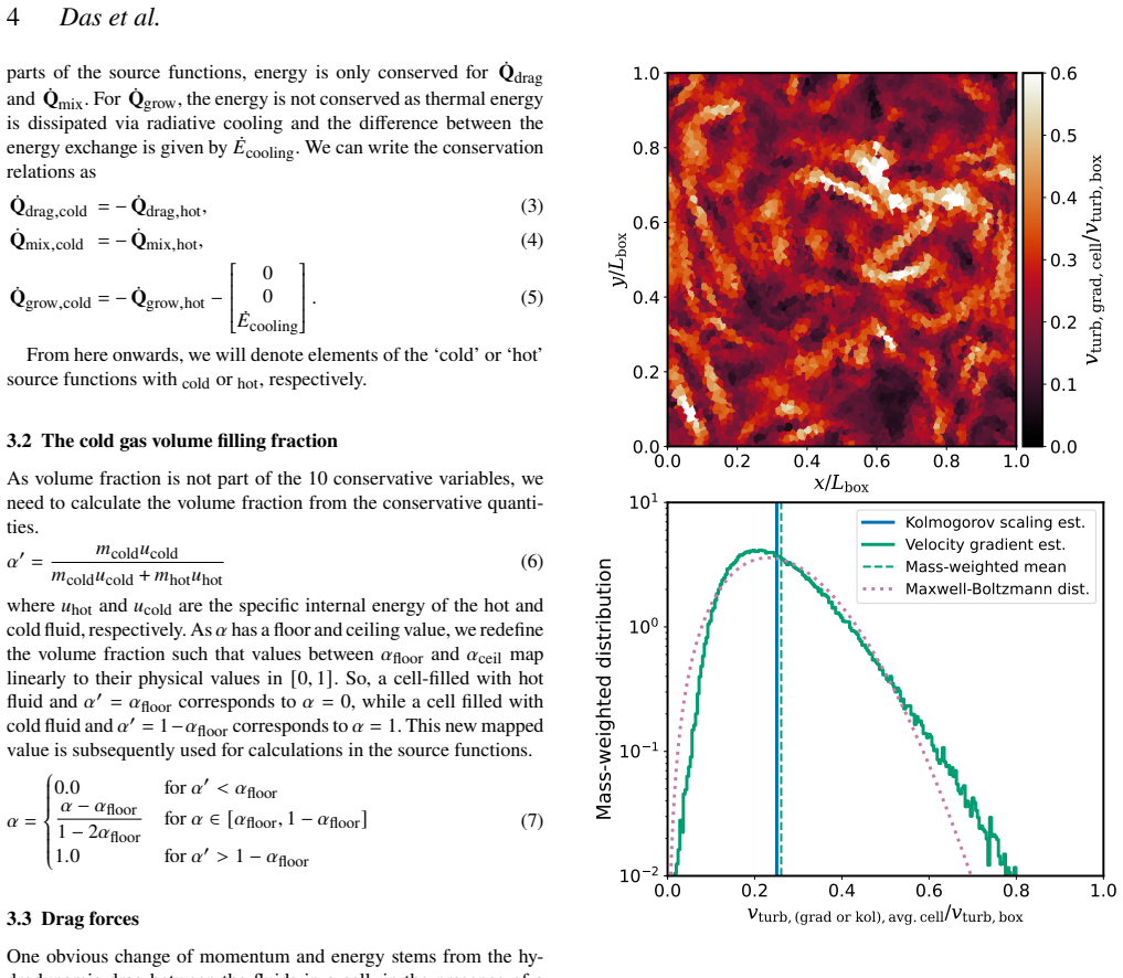
- The gradient-based velocity estimator could be reused as a general subgrid turbulence proxy in other multi-fluid codes, since it only needs the local velocity Jacobian; the paper notes slope-limiting distorts high-velocity tails, so accuracy in strongly shocked flows is an open question.
- The model's shielding threshold ($\alpha_{\rm mass}=0.15$) acts like a per-cell switch between destruction and growth; a similar switch might be needed in three-phase extensions (molecular-cold-hot), but the paper leaves that to future work.
Signed reviews
Editorial analysis
A structured set of objections, weighed in public.
Referee Report
Summary. Das, Gronke, and Weinberger present MOGLI, a subgrid model for unresolved cold gas implemented in the multifluid extension of AREPO. The model evolves hot and cold fluids with source terms for three physical processes: drag, turbulent mixing of cold into hot gas, and cold-gas growth by cooling of mixed gas. Local turbulent velocities are estimated either by Kolmogorov scaling from the box scale or locally from velocity gradients. The cold-gas surface area and cross-sectional area are represented through Monte-Carlo fits for ensembles of overlapping spheres. The paper verifies both a reduced non-radiative version and the full radiative version of the model against resolved Athena++ turbulent-box simulations, varying Mach number, spatial resolution, initial cloud resolvedness, and turbulence seeds. The reported diagnostics include cold-gas destruction timescales, growth rates, the Gronke et al. (2022) survival criterion, and cold-gas dispersion. The paper closes with a demonstration of a 64^3-cell simulation containing 100 unresolved clouds, which the authors argue would require roughly 3000^3 cells in a resolved single-fluid calculation.
Significance. The model addresses a real and widely recognized need: cosmological and galaxy-scale simulations cannot resolve the small cold clouds observed in galactic halos, and current simulations are non-converged in cold-gas content. The manuscript's main strength is its extensive verification suite: it tests a reduced model and the full model, compares two independent local-turbulence estimators, uses quantitative diagnostics (t_half, t_grow, survival, dispersion) across Mach number, resolution, resolvedness, and random seeds, and contains an honest discussion of limitations. The implementation in a widely used code and the small number of free parameters are additional assets. The main caveats are that the two free parameters are selected using the same benchmark class used for validation, and that the survival criterion is in large part a consistency check with the growth/destruction theory built into the model. If the calibration/validation distinction is addressed, the model would be a valuable tool for future large-scale multiphase simulations.
major comments (4)
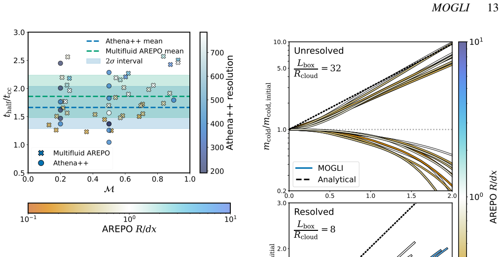
- [Secs. 3.4 and 5; Eqs. (15) and (29)] The two model parameters are calibrated against the same benchmark suite used for validation: alpha_mass=0.15 is introduced because it 'works well across all tests' (Sec. 3.4), and xi=2 is selected during the non-radiative mixing tests by comparing with benchmark Athena++ runs (Sec. 5). Consequently, the agreement in Figs. 7, 11, and 12 is partly in-sample fitting rather than independent prediction. To support the abstract's claim of predictive verification, the paper should provide a sensitivity scan over alpha_mass and xi and/or perform a holdout exercise in which one portion of the parameter space is used for calibration and the remainder for validation. The discussion should also clearly separate calibrated quantities from genuinely out-of-sample predictions.
- [Sec. 4.2.2; Eqs. (17) and (34)] The per-cell growth timescale in Eq. (17) is built from the same theoretical framework that produces the analytical global growth rate in Eq. (34), and the Monte-Carlo area factor is explicitly introduced to reproduce the 0.5 fudge factor from Gronke et al. (2022). Therefore Fig. 11 and the survival criterion in Fig. 12 verify the internal consistency of the implemented rates rather than an emergent, independent prediction. The paper should either identify a genuinely independent prediction not used in calibration or reframe the survival criterion as a consistency check rather than an emergent result.
- [Sec. 4.2.3; Figs. 13 and 18] Cold-gas dispersion is a diagnostic directly relevant to the intended applications, and the MOGLI runs overpredict it substantially: in the unresolved initial-cloud case, the normalized dispersion reaches roughly 10^4 at t = 2.5 t_eddy while the Athena++ benchmarks reach roughly 10^2, and the resolved case also shows a systematic offset. The text attributes this difference to numerical diffusion, but the abstract's statement of 'very good quantitative agreement across the different simulation parameters and diagnostics' and the conclusion bullet that dispersion is 'similar' are too strong. Please either reduce the discrepancy or quantify and qualify the claim, reporting absolute as well as normalized dispersion.
- [Sec. 3.7; Eqs. (30) and (33)] The interface-area and cross-sectional-area relations are derived from ensembles of overlapping spheres, and the validation benchmarks are initialized with spherical clouds. If the unresolved cold gas is filamentary or has a different area-volume relation, the mixing and growth rates in Eqs. (15) and (18) would change. Since the intended applications include small, potentially elongated cold structures in the CGM, the paper should either provide a sensitivity test with non-spherical initial morphologies or explicitly state this geometric assumption as a central limitation rather than implying general validity.
minor comments (6)
- [Fig. 8 and Sec. 4.2.1] The text describing the right two columns of Fig. 8 labels the resolved-cloud case as L_box/R_cloud = 32, but Sec. 4.1 and the surrounding discussion use L_box/R_cloud = 8 for resolved clouds; this is inconsistent and should be corrected.
- [Sec. 3.7, Eq. (30)] For a single non-overlapping sphere the geometric limit is A R/(2V) = 1.5 alpha, whereas Eq. (30) gives h=1 in the dilute limit, which corresponds to A R/(2V) = alpha; a sentence clarifying how the Monte-Carlo fit treats overlapping spheres and how the normalization was chosen would help.
- [Sec. 3.5, Eq. (17)] The origin of the alpha^(1/9) factor in Eq. (17) is not derived in the text; a one-sentence justification or a reference for this scaling would improve readability.
- [Sec. 2.3] The quasi-isothermal EOS for the cold fluid, which resets the internal energy after each timestep, is a significant approximation; its effect on the energy-exchanging source terms in Eqs. (11) and (16) should be discussed or tested.
- [Sec. 3.6.2, Eqs. (24)-(27)] The derivation of the velocity-gradient estimator assumes a uniform distribution of neighbours and roughly equal neighbour distances; the manuscript would benefit from a quantitative error estimate beyond the factor-of-two statement in the caption of Fig. 3.
- [Sec. 6.4] The possible sensitivity of the area and cross-section fits (Sec. 3.7) to non-spherical subgrid morphology is not listed among the limitations; given the intended CGM applications, this deserves explicit mention in the limitations section.
Circularity Check
Two calibrated parameters and the imported same-form growth rate make part of the benchmark agreement in-sample; independent diagnostics remain.
-
fitted input called prediction
[Sec. 3.6.3, Eq. (29), and Sec. 5 / Fig. 14]
"During our non-radiative turbulent mixing tests, explained later in Sec. 5, we find a ξ = 2 works better in matching with the benchmark Athena++ simulations. Hence, we use ξ = ξMOGLI≡ 2 in MOGLI runs"
ξ is a free normalization of the velocity-gradient turbulence estimator. It is chosen by matching the same non-radiative benchmark Athena++ simulations that Sec. 5 then presents as verification of the grad method. In particular, the t_half/t_cc scatter in Fig. 14 is in-sample for this parameter, so the stated agreement of the destruction timescale is partly a calibration result rather than an independent prediction.
-
fitted input called prediction
[Sec. 3.4, Eq. (15), and Sec. 4.1 / Figs. 6–7]
"The effect is that the mass exchange from cold to hot occurs only in cells that possess a mass fraction αmass less than a threshold. We find that a αmass threshold of 0.15 works well across all tests (§ 4.1), i.e., ṁcold→hot = {2h(α) mcold/tdestroy αmass < 0.15; 0 otherwise. (15)"
The αmass = 0.15 cutoff is a free parameter introduced to suppress mixing in cold-dominated cells. Its only stated calibration is that it 'works well across all tests (§ 4.1)', and those tests are the very resolved Athena++ non-radiative runs used as the destruction-timescale benchmark. Consequently, the t_half/t_cc agreement reported for the reduced model includes a parameter tuned to that comparison; it is not a clean out-of-sample verification of the mixing rate.
1 more flagged steps
-
self definitional
[Sec. 3.5 Eq. (17); Sec. 4.2.2 Eq. (34); Figs. 10–11]
"We can rewrite the expression for tgrow in terms of the local cell properties as, tgrow = χ(tdestroy tcool,cold)^{1/2} α^{1/9} (17) ... The analytical growth timescale, tgrow,theory, is given by (Gronke et al. 2022) tgrow,theory/tcc = 0.5χ(tcool,cold/tcc)^{1/2}(Lbox/Rcloud)^{1/6} (34). Note that while this equation is of the same form as the implemented Eq. (17), on a per-cell basis, it is important to point out that whether our simulations recover the correct global growth rate is far from obvious."
Equation (17) is presented as the cell-level form of the same Gronke et al. (2022) growth law that later defines the 'analytical' growth timescale in Eq. (34). MOGLI evolves exactly this per-cell growth source, so the near-unity tgrow/tgrow,theory ratios in Figs. 10–11 and 15–16 largely verify that the implementation returns the formula that was put into it. The benchmark also includes the resolved simulations of Gronke et al. (2022) and Das & Gronke (2024), the same body of work from which the growth rate was imported. The growth-rate agreement is therefore a consistency check, not an independent first-principles confirmation.
full rationale
The strongest circularity is concentrated in the two free parameters and the imported growth law. ξ = 2 and αmass = 0.15 are both calibrated against the resolved Athena++ turbulent-box simulations, and the same simulations are then used as the benchmark for the destruction-timescale and growth-rate verification. The growth timescale comparison is additionally weakened by the paper's own admission that Eq. (34) is 'of the same form' as the implemented Eq. (17); the subgrid growth term is effectively the analytical growth law repackaged per cell, so recovering that law in Figs. 10–11 is partly built in. The survival criterion is not explicitly coded, so its reproduction has some emergent content, but because the growth and destruction rates that determine survival were imported from the same Gronke et al. (2022) theory and benchmark set, it functions more as an internal consistency check than as an independent prediction. I do not rate the paper as wholly circular: the multifluid AREPO implementation, the geometric Monte-Carlo area factors, and the drag formulation are independently constructed, and the cold-gas dispersion diagnostic (Fig. 13) is a comparatively independent test that shows only qualitative agreement, with MOGLI over-predicting dispersion. The central quantitative claims of reproduction are nonetheless partially in-sample, giving a circularity score of 6 rather than a lower score.
Assumptions & free parameters
free parameters (2)
- alpha_mass mixing threshold =
0.15
- xi_MOGLI gradient normalization =
2
assumptions (7)
- domain assumption Multifluid hydrodynamics in AREPO (Weinberger & Hernquist 2023) accurately describes two compressible fluids sharing a grid.
- domain assumption The Bader-Deuflhard semi-implicit integrator (Weinberger et al., in prep) stably integrates the MOGLI source terms over a timestep.
- domain assumption Cold gas destruction timescale t_destroy = chi^(1/2) l_cold / v_turb (Eq. 12) from cloud-crushing theory and resolved simulations (Klein et al. 1994; Gronke et al. 2022) holds at the subgrid cell level.
- domain assumption Cold gas growth timescale t_grow = chi (t_destroy t_cool,cold)^(1/2) alpha^(1/9) (Eq. 17) from combustion-theory-derived resolved simulations (Tan et al. 2021; Gronke et al. 2022) holds per cell.
- domain assumption A fully developed Kolmogorov cascade extends from the box scale down to subgrid cold-gas scales (Eq. 21 and Sec. 3.6).
- ad hoc to paper Cold gas within a cell can be treated as an effective sphere with size l_cold=(alpha V_cell/(4 pi/3))^(1/3) and with surface area given by the overlapping-sphere Monte Carlo relation 2 h(alpha) (Sec. 3.7, Eq. 30).
- domain assumption Quasi-isothermal EOS for the cold fluid emulates the temperature floor and fast cooling of resolved single-fluid runs (Sec. 2.3).
Cite this review
Pith. "Pith review of MOGLI: Model for Multiphase Gas using Multifluid hydrodynamics." pith.science (2026). https://pith.science/paper/YJBCBTVK
@misc{pith2026241203751,
  author       = {Pith},
  title        = {Pith review of: MOGLI: Model for Multiphase Gas using Multifluid hydrodynamics},
  year         = {2026},
  howpublished = {\url{https://pith.science/paper/YJBCBTVK}},
  note         = {Machine review of arXiv:2412.03751}
}
abstract
Multiphase gas, with hot ($\sim10^6$K) and cold ($\sim10^4$K) gas, is ubiquitous in astrophysical media across a wide range of scales. However, simulating multiphase gas has been a long-standing challenge, due to the large separation between the size of cold gas structures and the scales at which such gas impacts the evolution of associated systems. In this study, we introduce a new subgrid framework for such multiphase gas, MOGLI: Model for Multiphase Gas using Multifluid hydrodynamics, in multifluid AREPO. We develop this approach based on first principles and theoretical results from previous studies with resolved small-scale simulations, leading to a minimal number of free parameters in the formulation. We divide the interactions in the model into three sources: drag, turbulent mixing and cold gas growth. As part of the model, we also include two methods for estimating the local turbulent velocities, one using the Kolmogorov scaling, and the other using the local velocity gradients. We verify the different components of the framework through extensive comparison with benchmark single-fluid simulations across different simulation parameters, such as how resolved the cold gas is initially, the turbulent Mach number, spatial resolution, and random initialisation of turbulence. We test the complete scheme and a reduced version, with and without cold gas growth. We find a very good qualitative and quantitative agreement across the different simulation parameters and diagnostics for both local turbulent velocity estimation methods. We also reproduce behaviour like the cold gas survival criteria as an emergent property. We discuss the applications and possible extensions of MOGLI and demonstrate its capability by running a simulation which would be computationally prohibitive to run as a resolved single-fluid simulation.
Figures


Figures from the paper (14 more)




Forward citations
Cited by 2 Pith papers
-
Woven by the Whirls: The growth and entrainment of cold clouds in turbulent hot winds
Subsonic turbulence in a hot wind enlarges the cloud–wind mixing surface, boosting cold-cloud mass growth up to ~10× when cooling is fast and shortening entrainment time.
-
The Synthetic Absorption Line Spectral Almanac (SALSA)
A new public library generates millions of mock quasar absorption spectra from cosmological simulations, using a novel mesh-free Voronoi ray-tracing algorithm.
Reference graph
Works this paper leans on
-
[1]
write newline
" write newline "" before.all 'output.state := FUNCTION fin.entry write newline FUNCTION new.block output.state before.all = 'skip after.block 'output.state := if FUNCTION new.sentence output.state after.block = 'skip output.state before.all = 'skip after.sentence 'output.state := if if FUNCTION not #0 #1 if FUNCTION and 'skip pop #0 if FUNCTION or pop #1...
-
[2]
Abruzzo M. W., Fielding D. B., Bryan G. L., 2024, @doi [ ] 10.3847/1538-4357/ad1e51 , https://ui.adsabs.harvard.edu/abs/2024ApJ...966..181A 966, 181
-
[3]
Armillotta L., Fraternali F., Marinacci F., 2016, @doi [Monthly Notices of the Royal Astronomical Society] 10.1093/mnras/stw1930 , 462, 4157
-
[4]
Audit E., Hennebelle P., 2005, @doi [A&A] 10.1051/0004-6361:20041474 , 433, 1
-
[5]
Bader G., Deuflhard P., 1983, Numerische Mathematik, 41, 373
1983
-
[6]
C., Fabian A
Begelman M. C., Fabian A. C., 1990, , https://ui.adsabs.harvard.edu/abs/1990MNRAS.244P..26B 244, 26P
1990
-
[7]
Berczik P., Hensler G., Theis C., Spurzem R., 2003, @doi [Astrophysics and Space Science] 10.1023/A:1024085909715 , 284, 865
-
[8]
Butsky I. S., Fielding D. B., Hayward C. C., Hummels C. B., Quinn T. R., Werk J. K., 2020, @doi [The Astrophysical Journal] 10.3847/1538-4357/abbad2 , 903, 77
Show all 95 references
-
[9]
S., Hummels C
Butsky I. S., Hummels C. B., Hopkins P. F., Quinn T. R., Werk J. K., 2024, @doi [ ] 10.1093/mnras/stae2459 , https://ui.adsabs.harvard.edu/abs/2024MNRAS.535.1672B 535, 1672
2024 doi
-
[10]
Clarendon Press
Chandrasekhar S., 1961, Hydrodynamic and hydromagnetic stability . Clarendon Press
1961
-
[11]
Chang S.-J., Gronke M., 2024, @doi [ ] 10.1093/mnras/stae1664 , https://ui.adsabs.harvard.edu/abs/2024MNRAS.532.3526C 532, 3526
2024 doi
-
[12]
P., 2024, @doi [Monthly Notices of the Royal Astronomical Society] 10.1093/mnras/stae1113 , 530, 4032
Chen Z., Oh S. P., 2024, @doi [Monthly Notices of the Royal Astronomical Society] 10.1093/mnras/stae1113 , 530, 4032
2024 doi
-
[13]
Chen H.-W., et al., 2023, @doi [ ] 10.3847/2041-8213/acf85b , https://ui.adsabs.harvard.edu/abs/2023ApJ...955L..25C 955, L25
2023 doi
-
[14]
P., Sharma P., Quataert E., 2019, @doi [Monthly Notices of the Royal Astronomical Society] 10.1093/mnras/stz1857 , 488, 3195
Choudhury P. P., Sharma P., Quataert E., 2019, @doi [Monthly Notices of the Royal Astronomical Society] 10.1093/mnras/stz1857 , 488, 3195
2019 doi
-
[16]
Crighton N. H. M., Hennawi J. F., Simcoe R. A., Cooksey K. L., Murphy M. T., Fumagalli M., Prochaska J. X., Shanks T., 2015, @doi [Monthly Notices of the Royal Astronomical Society] 10.1093/mnras/stu2088 , 446, 18
2015 doi
-
[17]
K., Gronke M., 2024, @doi [ ] 10.1093/mnras/stad3125 , https://ui.adsabs.harvard.edu/abs/2024MNRAS.527..991D 527, 991
Das H. K., Gronke M., 2024, @doi [ ] 10.1093/mnras/stad3125 , https://ui.adsabs.harvard.edu/abs/2024MNRAS.527..991D 527, 991
2024 doi
-
[18]
K., Choudhury P
Das H. K., Choudhury P. P., Sharma P., 2021, @doi [Monthly Notices of the Royal Astronomical Society] 10.1093/mnras/stab382 , 502, 4935
2021 doi
-
[19]
M., 2022, @doi [ ] 10.1016/j.physrep.2022.04.005 , https://ui.adsabs.harvard.edu/abs/2022PhR...973....1D 973, 1
Donahue M., Voit G. M., 2022, @doi [ ] 10.1016/j.physrep.2022.04.005 , https://ui.adsabs.harvard.edu/abs/2022PhR...973....1D 973, 1
2022 doi
-
[20]
Eswaran V., Pope S., 1988, @doi [Computers & Fluids] https://doi.org/10.1016/0045-7930(88)90013-8 , 16, 257
1988 doi
-
[21]
J., Gronke M., 2021, arXiv e-prints, 17, 1
Farber R. J., Gronke M., 2021, arXiv e-prints, 17, 1
2021
-
[22]
P., 2023, @doi [ ] 10.1146/annurev-astro-052920-125203 , https://ui.adsabs.harvard.edu/abs/2023ARA&A..61..131F 61, 131
Faucher-Gigu \`e re C.-A., Oh S. P., 2023, @doi [ ] 10.1146/annurev-astro-052920-125203 , https://ui.adsabs.harvard.edu/abs/2023ARA&A..61..131F 61, 131
2023 doi
-
[23]
S., 2012, @doi [ ] 10.1088/0004-637X/761/2/156 , https://ui.adsabs.harvard.edu/abs/2012ApJ...761..156F 761, 156
Federrath C., Klessen R. S., 2012, @doi [ ] 10.1088/0004-637X/761/2/156 , https://ui.adsabs.harvard.edu/abs/2012ApJ...761..156F 761, 156
2012 doi
-
[24]
B., Field G
Field G. B., Field G. B., 1965, The Astrophysical Journal, pp 531--567
1965
-
[25]
B., Ostriker E
Fielding D. B., Ostriker E. C., Bryan G. L., Jermyn A. S., 2020, @doi [The Astrophysical Journal] 10.3847/2041-8213/ab8d2c , 894, L24
2020 doi
-
[26]
Gronke M., Peng Oh S., 2018, @doi [Monthly Notices of the Royal Astronomical Society: Letters] 10.1093/mnrasl/sly131 , 480, L111
2018 doi
-
[27]
P., 2016, @doi [ ] 10.3847/2041-8213/833/2/L26 , https://ui.adsabs.harvard.edu/abs/2016ApJ...833L..26G 833, L26
Gronke M., Dijkstra M., McCourt M., Oh S. P., 2016, @doi [ ] 10.3847/2041-8213/833/2/L26 , https://ui.adsabs.harvard.edu/abs/2016ApJ...833L..26G 833, L26
2016 doi
-
[28]
P., Ji S., Norman C., 2022, @doi [ ] 10.1093/mnras/stab3351 , https://ui.adsabs.harvard.edu/abs/2022MNRAS.511..859G 511, 859
Gronke M., Oh S. P., Ji S., Norman C., 2022, @doi [ ] 10.1093/mnras/stab3351 , https://ui.adsabs.harvard.edu/abs/2022MNRAS.511..859G 511, 859
2022 doi
-
[30]
Harfst S., Theis C., Hensler G., 2004, @doi [Publications of the Astronomical Society of Australia] 10.1071/AS04020 , 21, 228
2004 doi
-
[31]
R., et al., 2020, @doi [Nature] 10.1038/s41586-020-2649-2 , 585, 357
Harris C. R., et al., 2020, @doi [Nature] 10.1038/s41586-020-2649-2 , 585, 357
2020 doi
- [32]
-
[33]
J., Gronke M., 2024, @doi [ ] 10.1093/mnras/stad3069 , https://ui.adsabs.harvard.edu/abs/2024MNRAS.527..135H 527, 135
Hidalgo-Pineda F., Farber R. J., Gronke M., 2024, @doi [ ] 10.1093/mnras/stad3069 , https://ui.adsabs.harvard.edu/abs/2024MNRAS.527..135H 527, 135
2024 doi
-
[34]
H., Peeples M
Huang S., Katz N., Scannapieco E., Cottle J., Dav \'e R., Weinberg D. H., Peeples M. S., Br \"u ggen M., 2020, @doi [ ] 10.1093/mnras/staa1978 , https://ui.adsabs.harvard.edu/abs/2020MNRAS.497.2586H 497, 2586
2020 doi
-
[35]
B., Smith B
Hummels C. B., Smith B. D., Silvia D. W., 2017, @doi [The Astrophysical Journal] 10.3847/1538-4357/aa7e2d , 847, 59
2017 doi
-
[36]
B., et al., 2019, @doi [The Astrophysical Journal] 10.3847/1538-4357/ab378f , 882, 156
Hummels C. B., et al., 2019, @doi [The Astrophysical Journal] 10.3847/1538-4357/ab378f , 882, 156
2019 doi
-
[37]
B., Rubin K
Hummels C. B., Rubin K. H. R., Schneider E. E., Fielding D. B., 2024, @doi [ ] 10.3847/1538-4357/ad5965 , https://ui.adsabs.harvard.edu/abs/2024ApJ...972..148H 972, 148
2024 doi
-
[38]
D., 2007, @doi [Computing in Science & Engineering] 10.1109/MCSE.2007.55 , 9, 90
Hunter J. D., 2007, @doi [Computing in Science & Engineering] 10.1109/MCSE.2007.55 , 9, 90
2007 doi
-
[39]
P., Masterson P., 2019, @doi [Monthly Notices of the Royal Astronomical Society] 10.1093/mnras/stz1248 , 487, 737
Ji S., Oh S. P., Masterson P., 2019, @doi [Monthly Notices of the Royal Astronomical Society] 10.1093/mnras/stz1248 , 487, 737
2019 doi
-
[40]
Kanjilal V., Dutta A., Sharma P., 2021, @doi [Monthly Notices of the Royal Astronomical Society] 10.1093/mnras/staa3610 , 501, 1143
2021 doi
-
[41]
Kannan R., Garaldi E., Smith A., Pakmor R., Springel V., Vogelsberger M., Hernquist L., 2022, @doi [Monthly Notices of the Royal Astronomical Society] 10.1093/mnras/stab3710 , 511, 4005
2022 doi
-
[42]
C., 2015, @doi [ ] 10.1088/0004-637X/802/2/99 , https://ui.adsabs.harvard.edu/abs/2015ApJ...802...99K 802, 99
Kim C.-G., Ostriker E. C., 2015, @doi [ ] 10.1088/0004-637X/802/2/99 , https://ui.adsabs.harvard.edu/abs/2015ApJ...802...99K 802, 99
2015 doi
-
[43]
C., 2017, @doi [ ] 10.3847/1538-4357/aa8599 , https://ui.adsabs.harvard.edu/abs/2017ApJ...846..133K 846, 133
Kim C.-G., Ostriker E. C., 2017, @doi [ ] 10.3847/1538-4357/aa8599 , https://ui.adsabs.harvard.edu/abs/2017ApJ...846..133K 846, 133
2017 doi
-
[44]
I., McKee C
Klein R. I., McKee C. F., Colella P., 1994, @doi [ ] 10.1086/173554 , https://ui.adsabs.harvard.edu/abs/1994ApJ...420..213K 420, 213
1994 doi
-
[45]
Lan T.-W., Fukugita M., 2017, @doi [ ] 10.3847/1538-4357/aa93eb , https://ui.adsabs.harvard.edu/abs/2017ApJ...850..156L 850, 156
2017 doi
-
[46]
Ledos N., Takasao S., Nagamine K., 2024, @doi [ ] 10.1093/mnras/stad3814 , https://ui.adsabs.harvard.edu/abs/2024MNRAS.52711304L 527, 11304
2024 doi
-
[47]
H., Roberts W
Levinson F. H., Roberts W. W. J., 1981, @doi [ ] 10.1086/158823 , https://ui.adsabs.harvard.edu/abs/1981ApJ...245..465L 245, 465
1981 doi
-
[48]
E., Cline H
Lorensen W. E., Cline H. E., 1987, in Proceedings of the 14th Annual Conference on Computer Graphics and Interactive Techniques. SIGGRAPH '87. Association for Computing Machinery, New York, NY, USA, p. 163–169, @doi 10.1145/37401.37422 , https://doi.org/10.1145/37401.37422
1987
-
[49]
C., 2020, @doi [Monthly Notices of the Royal Astronomical Society] 10.1093/mnras/staa812 , 494, 2641
Mandelker N., Nagai D., Aung H., Dekel A., Birnboim Y., van den Bosch F. C., 2020, @doi [Monthly Notices of the Royal Astronomical Society] 10.1093/mnras/staa812 , 494, 2641
2020 doi
-
[50]
Martizzi D., Fielding D., Faucher-Gigu \`e re C.-A., Quataert E., 2016, @doi [ ] 10.1093/mnras/stw745 , https://ui.adsabs.harvard.edu/abs/2016MNRAS.459.2311M 459, 2311
2016 doi
-
[51]
P., O'Leary R., Madigan A.-M., 2018, @doi [Monthly Notices of the Royal Astronomical Society] 10.1093/mnras/stx2687 , 473, 5407
McCourt M., Oh S. P., O'Leary R., Madigan A.-M., 2018, @doi [Monthly Notices of the Royal Astronomical Society] 10.1093/mnras/stx2687 , 473, 5407
2018 doi
-
[52]
F., Ostriker J
McKee C. F., Ostriker J. P., 1977, @doi [The Astrophysical Journal] 10.1086/155667 , 218, 148
1977 doi
-
[54]
Mohapatra R., Federrath C., Sharma P., 2020, @doi [Monthly Notices of the Royal Astronomical Society] 10.1093/mnras/staa711 , 493, 5838
2020 doi
-
[55]
Mohapatra R., Jetti M., Sharma P., Federrath C., 2022, @doi [Monthly Notices of the Royal Astronomical Society] 10.1093/mnras/stab3603 , 510, 3778
2022 doi
-
[56]
P., 2017, @doi [ ] 10.1146/annurev-astro-081913-040019 , https://ui.adsabs.harvard.edu/abs/2017ARA&A..55...59N 55, 59
Naab T., Ostriker J. P., 2017, @doi [ ] 10.1146/annurev-astro-081913-040019 , https://ui.adsabs.harvard.edu/abs/2017ARA&A..55...59N 55, 59
2017 doi
-
[57]
R., Frenk C
Okamoto T., Eke V. R., Frenk C. S., Jenkins A., 2005, @doi [ ] 10.1111/j.1365-2966.2005.09525.x , https://ui.adsabs.harvard.edu/abs/2005MNRAS.363.1299O 363, 1299
2005
-
[59]
J., Ohlmann S
Pakmor R., Springel V., Bauer A., Mocz P., Munoz D. J., Ohlmann S. T., Schaal K., Zhu C., 2016, @doi [ ] 10.1093/mnras/stv2380 , https://ui.adsabs.harvard.edu/abs/2016MNRAS.455.1134P 455, 1134
2016 doi
-
[60]
Pedregosa F., et al., 2011, Journal of Machine Learning Research, 12, 2825
2011
-
[61]
S., et al., 2019, @doi [ ] 10.3847/1538-4357/ab0654 , https://ui.adsabs.harvard.edu/abs/2019ApJ...873..129P 873, 129
Peeples M. S., et al., 2019, @doi [ ] 10.3847/1538-4357/ab0654 , https://ui.adsabs.harvard.edu/abs/2019ApJ...873..129P 873, 129
2019 doi
-
[62]
C., 2020, @doi [Annual Review of Astronomy and Astrophysics] 10.1146/annurev-astro-021820-120014 , 58, 363
P \' e roux C., Howk J. C., 2020, @doi [Annual Review of Astronomy and Astrophysics] 10.1146/annurev-astro-021820-120014 , 58, 363
2020 doi
-
[63]
Cambridge University Press
Prosperetti A., Tryggvason G., 2007, Computational Methods for Multiphase Flow. Cambridge University Press
2007
-
[64]
Ramesh R., Nelson D., 2024, @doi [ ] 10.1093/mnras/stae237 , https://ui.adsabs.harvard.edu/abs/2024MNRAS.528.3320R 528, 3320
2024 doi
-
[65]
Rauch M., Sargent W. L. W., Barlow T. A., 1999, @doi [ ] 10.1086/307060 , https://ui.adsabs.harvard.edu/abs/1999ApJ...515..500R 515, 500
1999 doi
-
[66]
Rosdahl J., Schaye J., Dubois Y., Kimm T., Teyssier R., 2017, @doi [ ] 10.1093/mnras/stw3034 , https://ui.adsabs.harvard.edu/abs/2017MNRAS.466...11R 466, 11
2017 doi
-
[67]
C., Steidel C
Rudie G. C., Steidel C. C., Pettini M., Trainor R. F., Strom A. L., Hummels C. B., Reddy N. A., Shapley A. E., 2019, @doi [ ] 10.3847/1538-4357/ab4255 , https://ui.adsabs.harvard.edu/abs/2019ApJ...885...61R 885, 61
2019 doi
-
[68]
Saurel R., Abgrall R., 1999, @doi [Journal of Computational Physics] https://doi.org/10.1006/jcph.1999.6187 , 150, 425
1999
-
[69]
Scannapieco E., Br \"u ggen M., 2008, @doi [ ] 10.1086/591228 , https://ui.adsabs.harvard.edu/abs/2008ApJ...686..927S 686, 927
2008 doi
-
[70]
B., White S
Scannapieco C., Tissera P. B., White S. D., Springel V., 2006, @doi [Monthly Notices of the Royal Astronomical Society] 10.1111/j.1365-2966.2006.10785.x , 371, 1125
2006
-
[71]
F., Kim T.-S., 2007, @doi [ ] 10.1111/j.1365-2966.2007.12005.x , https://ui.adsabs.harvard.edu/abs/2007MNRAS.379.1169S 379, 1169
Schaye J., Carswell R. F., Kim T.-S., 2007, @doi [ ] 10.1111/j.1365-2966.2007.12005.x , https://ui.adsabs.harvard.edu/abs/2007MNRAS.379.1169S 379, 1169
2007
-
[72]
Schmidt W., Federrath C., 2011, @doi [ ] 10.1051/0004-6361/201015630 , https://ui.adsabs.harvard.edu/abs/2011A&A...528A.106S 528, A106
2011 doi
-
[73]
C., Hillebrandt W., 2006, @doi [ ] 10.1051/0004-6361:20053617 , https://ui.adsabs.harvard.edu/abs/2006A&A...450..265S 450, 265
Schmidt W., Niemeyer J. C., Hillebrandt W., 2006, @doi [ ] 10.1051/0004-6361:20053617 , https://ui.adsabs.harvard.edu/abs/2006A&A...450..265S 450, 265
2006 doi
-
[74]
Semelin B., Combes F., 2002, @doi [Astronomy & Astrophysics] 10.1051/0004-6361:20020547 , 388, 826
2002 doi
-
[75]
A., 2024, @doi [arXiv e-prints] 10.48550/arXiv.2410.23339 , https://ui.adsabs.harvard.edu/abs/2024arXiv241023339S p
Semenov V. A., 2024, @doi [arXiv e-prints] 10.48550/arXiv.2410.23339 , https://ui.adsabs.harvard.edu/abs/2024arXiv241023339S p. arXiv:2410.23339
2024 doi
-
[76]
J., Quataert E., 2010, @doi [Astrophysical Journal] 10.1088/0004-637X/720/1/652 , 720, 652
Sharma P., Parrish I. J., Quataert E., 2010, @doi [Astrophysical Journal] 10.1088/0004-637X/720/1/652 , 720, 652
2010 doi
-
[77]
J., 2012, @doi [Monthly Notices of the Royal Astronomical Society] 10.1111/j.1365-2966.2011.20246.x , 420, 3174
Sharma P., Mccourt M., Quataert E., Parrish I. J., 2012, @doi [Monthly Notices of the Royal Astronomical Society] 10.1111/j.1365-2966.2011.20246.x , 420, 3174
2012
-
[78]
B., 2024, @doi [arXiv e-prints] 10.48550/arXiv.2411.17173 , https://ui.adsabs.harvard.edu/abs/2024arXiv241117173S p
Singh Bisht M., Sharma P., Duttta A., Nath B. B., 2024, @doi [arXiv e-prints] 10.48550/arXiv.2411.17173 , https://ui.adsabs.harvard.edu/abs/2024arXiv241117173S p. arXiv:2411.17173
-
[79]
C., Sijacki D., Shen S., 2018, @doi [ ] 10.1093/mnras/sty994 , https://ui.adsabs.harvard.edu/abs/2018MNRAS.478..302S 478, 302
Smith M. C., Sijacki D., Shen S., 2018, @doi [ ] 10.1093/mnras/sty994 , https://ui.adsabs.harvard.edu/abs/2018MNRAS.478..302S 478, 302
2018 doi
- [80]
-
[81]
C., 2019, @doi [Monthly Notices of the Royal Astronomical Society] 10.1093/mnras/stz792 , 486, 205
Sobacchi E., Sormani M. C., 2019, @doi [Monthly Notices of the Royal Astronomical Society] 10.1093/mnras/stz792 , 486, 205
2019 doi
-
[82]
Springel V., 2010, @doi [ ] 10.1111/j.1365-2966.2009.15715.x , https://ui.adsabs.harvard.edu/abs/2010MNRAS.401..791S 401, 791
2010
-
[83]
Springel V., Hernquist L., 2003, @doi [ ] 10.1046/j.1365-8711.2003.06206.x , https://ui.adsabs.harvard.edu/abs/2003MNRAS.339..289S 339, 289
2003
-
[84]
M., Tomida K., White C
Stone J. M., Tomida K., White C. J., Felker K. G., 2020, @doi [The Astrophysical Journal Supplement Series] 10.3847/1538-4365/ab929b , 249, 4
2020 doi
-
[85]
B., 2023, MNRAS, 000, 1
Tan B., Fielding D. B., 2023, MNRAS, 000, 1
2023
-
[86]
P., Gronke M., 2021, @doi [Monthly Notices of the Royal Astronomical Society] 10.1093/mnras/stab053 , 502, 3179
Tan B., Oh S. P., Gronke M., 2021, @doi [Monthly Notices of the Royal Astronomical Society] 10.1093/mnras/stab053 , 502, 3179
2021 doi
-
[87]
P., Gronke M., 2023, @doi [ ] 10.1093/mnras/stad236 , https://ui.adsabs.harvard.edu/abs/2023MNRAS.520.2571T 520, 2571
Tan B., Oh S. P., Gronke M., 2023, @doi [ ] 10.1093/mnras/stad236 , https://ui.adsabs.harvard.edu/abs/2023MNRAS.520.2571T 520, 2571
2023 doi
-
[88]
Townsend R. H. D., 2009, @doi [ ] 10.1088/0067-0049/181/2/391 , https://ui.adsabs.harvard.edu/abs/2009ApJS..181..391T 181, 391
2009 doi
-
[89]
S., Werk J
Tumlinson J., Peeples M. S., Werk J. K., 2017, @doi [Annual Review of Astronomy and Astrophysics] 10.1146/annurev-astro-091916-055240 , AA, 1
2017 doi
-
[90]
Veilleux S., Cecil G., Bland-Hawthorn J., 2005, @doi [Annual Review of Astronomy and Astrophysics] 10.1146/annurev.astro.43.072103.150610 , 43, 769
2005 arXiv
-
[91]
D., Aalto S., 2020, @doi [ ] 10.1007/s00159-019-0121-9 , https://ui.adsabs.harvard.edu/abs/2020A&ARv..28....2V 28, 2
Veilleux S., Maiolino R., Bolatto A. D., Aalto S., 2020, @doi [ ] 10.1007/s00159-019-0121-9 , https://ui.adsabs.harvard.edu/abs/2020A&ARv..28....2V 28, 2
2020 doi
-
[92]
Virtanen P., et al., 2020, @doi [Nature Methods] 10.1038/s41592-019-0686-2 , 17, 261
2020 doi
-
[93]
Walch S., et al., 2015, @doi [ ] 10.1093/mnras/stv1975 , https://ui.adsabs.harvard.edu/abs/2015MNRAS.454..238W 454, 238
2015 doi
-
[94]
P., Ruszkowski M., 2023, @doi [ ] 10.1093/mnras/stad003 , https://ui.adsabs.harvard.edu/abs/2023MNRAS.519.4408W 519, 4408
Wang C., Oh S. P., Ruszkowski M., 2023, @doi [ ] 10.1093/mnras/stad003 , https://ui.adsabs.harvard.edu/abs/2023MNRAS.519.4408W 519, 4408
2023 doi
-
[95]
Weinberger R., Hernquist L., 2023, @doi [ ] 10.1093/mnras/stac3708 , https://ui.adsabs.harvard.edu/abs/2023MNRAS.519.3011W 519, 3011
2023 doi
-
[96]
Weinberger R., Springel V., Pakmor R., 2020, @doi [ ] 10.3847/1538-4365/ab908c , https://ui.adsabs.harvard.edu/abs/2020ApJS..248...32W 248, 32
2020 doi
-
[97]
Wiersma R. P. C., Schaye J., Smith B. D., 2009, @doi [ ] 10.1111/j.1365-2966.2008.14191.x , https://ui.adsabs.harvard.edu/abs/2009MNRAS.393...99W 393, 99
2009
-
[98]
A., Grand R
van de Voort F., Bieri R., Pakmor R., G \' o mez F. A., Grand R. J. J., Marinacci F., 2021, @doi [Monthly Notices of the Royal Astronomical Society] 10.1093/mnras/staa3938 , 501, 4888
2021 doi
-
[99]
write newline
" write newline "" before.all 'output.state := FUNCTION fin.entry write newline FUNCTION new.block output.state before.all = 'skip after.block 'output.state := if FUNCTION new.sentence output.state after.block = 'skip output.state before.all = 'skip after.sentence 'output.stat...
Reviewed August 11, 2026 · model on record in the stance chip above.
Discussion (0). Continue with ORCID to comment.