REVIEW 5 major objections 6 minor 64 references
Monocular Dynamic Gaussian Splatting: Fast, Brittle, and Scene Complexity Rules
T0 review · 5 major / 6 minor · reviewed 2026-08-11 · deepseek-v4-flash
Pith's one-line read This benchmark of monocular dynamic Gaussian-splatting methods argues that the field's speed claims are real—20 to 200 frames per second—but that image quality is consistently beaten by a slower voxel-based method, TiNeuVox, and that…
desk verdict A genuinely useful reality-check benchmark for monocular dynamic Gaussian splatting, with one real caveat: the fairness of the cross-method comparison rests on an asserted but unshown reimplementation parity. read the letter →
The pith
A machine-rendered reading of the paper's core claim, the machinery that carries it, and where it could break.
The reading
What carries the argument
The central mechanism is a unified evaluation harness: five motion-representation families implemented in one codebase with shared hyperparameters, plus static 3DGS and the voxel-based TiNeuVox as baselines, run on a total of 50 scenes from five datasets and on a new instructive synthetic dataset. The synthetic dataset varies camera baseline B and object-motion distance D independently, isolating how each factor hurts reconstruction, while tracking-derived dynamic masks force separate measurement of quality on moving regions rather than letting static background dominate the metrics. This harness is what lets the paper attribute performance differences to motion representation rather than to dataset split or implementation details, and it is also what exposes the brittleness of adaptive density control.
What would settle it
Run the paper's five methods in their original released implementations with their original per-scene hyperparameters on the iPhone dataset and the narrow-baseline synthetic scenes, then compare masked LPIPS on dynamic regions; if a per-Gaussian method (EffGS or STG) or the 4D method RTGS beats DeformableGS and TiNeuVox, the paper's claims that field-based representations help and that scene complexity dominates would be contradicted.
Extended reading notes
Core claim
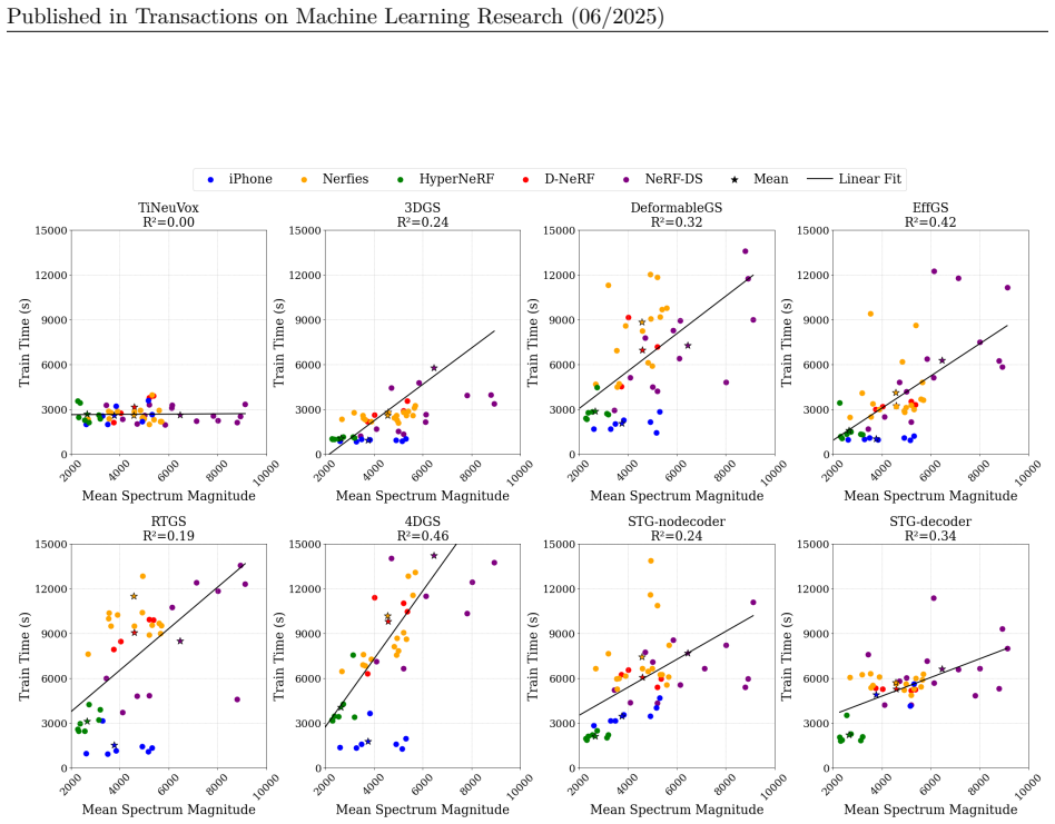
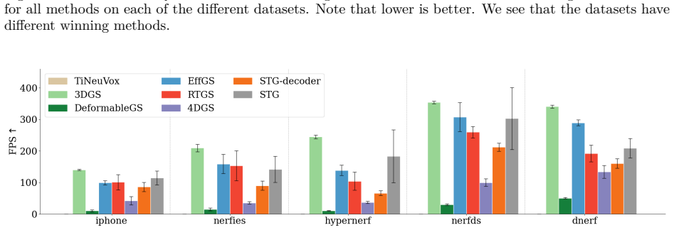
On the paper's own terms, the central discovery is that monocular dynamic Gaussian splatting is currently fast but brittle, and that scene difficulty rules. Averaged over five real-world datasets totaling 50 scenes, the non-Gaussian voxel method TiNeuVox reaches 24.54 PSNR while the best Gaussian method (DeformableGS) reaches 24.07, and TiNeuVox trains in comparable time and converges reliably; Gaussian methods render at 20–200 FPS versus TiNeuVox's 0.3 FPS. Among Gaussian methods, field-based motion representations (MLP or HexPlane) give better LPIPS than per-Gaussian low-order motion models, and the most expressive representation—direct 4D Gaussians—performs worst in both quality and efficiency. Yet across datasets the winning method changes, so no clear rank order emerges; on strictly-monocular iPhone data all Gaussian methods lag TiNeuVox by a wide margin. A controlled synthetic dataset shows reconstruction degrades as camera baseline shrinks or object motion grows, that static 3DGS can look competitive by reconstructing the background while inserting pseudo-dynamic Gaussians along a motion path, and that adaptive density control causes overfitting, varying efficiency, and occasional catastrophic optimization failures.
Load-bearing premise
The apples-to-apples comparison assumes that the integrated single-codebase reimplementations faithfully reproduce each original method, so the measured rank order reflects motion representation rather than implementation or hyperparameter differences.
Editorial extensions
If this is right
- Published claims that a new motion representation is universally best should be treated as unestablished unless the method is tested across datasets like D-NeRF, Nerfies, HyperNeRF, NeRF-DS, and iPhone with masked dynamic-region metrics.
- Field-based motion (shared MLP or HexPlane) is a safer default than per-Gaussian polynomial/Fourier motion or direct 4D Gaussians when scenes are monocular with narrow baselines.
- A static 3DGS baseline can look competitive on full-image metrics even when it fails on moving objects, so masked metrics on dynamic regions are necessary for meaningful comparison.
- Efficiency claims are not stable across scenes because adaptive density control produces very different Gaussian counts, so training and rendering times need per-scene reporting.
- TiNeuVox's quality advantage suggests that hybrid voxel-field representations remain a viable alternative to Gaussian splatting where rendering speed is not the priority.
Reading between the lines
- Editorial: The paper's measurements could be converted into a scalar scene-difficulty score combining baseline, motion magnitude, pose noise, and frequency content; if such a score predicted each method's error across the 50 scenes, benchmark findings would become transferable to new videos.
- Editorial: If scene complexity dominates method choice, an adaptive model selector that estimates baseline and motion speed from a video and then picks the motion representation could outperform any fixed choice; the paper's released data could train such a selector.
- Editorial: The paper's negative results for per-Gaussian and 4D methods should be read as "under uniform optimization," not "never works," because the shared-hyperparameter design is deliberate and a practitioner with per-scene tuning might obtain different rankings.
- Editorial: The brittleness of adaptive density control points to densification scheduling and regularization, rather than new motion representations, as likely sources of near-term progress in monocular dynamic Gaussian splatting.
Editorial analysis
A structured set of objections, weighed in public.
Referee Report
Summary. This manuscript benchmarks monocular dynamic view synthesis under Gaussian splatting. The authors collect 50 real-world scenes across D-NeRF, Nerfies, HyperNeRF, NeRF-DS, and iPhone, add a new synthetic dataset that varies camera baseline and object motion, and integrate five Gaussian methods (EffGS, STG, DeformableGS, 4DGS, RTGS) together with static 3DGS and TiNeuVox baselines into a shared codebase. They report three optimization runs per condition, standard deviations, and masked dynamic-region metrics. The paper's central thesis is that monocular dynamic Gaussian splatting is fast but brittle, that scene complexity and dataset factors overwhelm motion-representation differences, and that hybrid voxel/neural-field methods such as TiNeuVox remain competitive in quality. Eight findings summarize the evidence.
Significance. If the findings are correct, this is a useful and timely empirical contribution. Its strongest assets are the full-slate comparison on datasets where most original papers reported only subsets (Table 8), the controlled synthetic dataset with baseline/motion ablations, the use of three seeds and standard deviations, the masked static/dynamic metrics, and the public release of code and data. The paper is also appropriately candid about its limitations, including the lack of a method-independent scene-difficulty metric and the omission of concurrent works. The main risk to significance is reimplementation fidelity: the rank-order conclusions are only as trustworthy as the authors' integrated implementations, and that is not currently demonstrated.
major comments (5)
- [Sec. 4, first paragraph; Sec. 3.3; App. C.3; Table 2] The central assumption stated in Section 4, first paragraph, is that the integrated implementations 'approximately match the results of the original works', but the paper provides no parity table or quantitative evidence for this claim. This is especially consequential for STG: Section 3.3 and Appendix C.3 explain that STG was originally designed for multi-view input and had to be adapted for monocular input by copying the point cloud 10x along the time axis, and Table 2 reports a 4.56 dB gap between STG and DeformableGS (19.51 vs. 24.07). Because the qualitative conclusions are rank-order claims, even a 2-3 dB implementation gap on one method could change the story (compare TiNeuVox 24.54 and DeformableGS 24.07 in the same table). Please add a per-method, per-dataset parity check against the original papers' reported numbers on the scenes and splits they used, and justify or clearly separate the STG modifications and the STG/STG-decoder distinction.
- [Sec. 4.4; Table 2; Fig. 14] Section 4.4 states that collapsed optimization runs are excluded from the evaluation statistics, but the number, frequency, and location of these failures are never reported. This is load-bearing because Table 2 and Figure 5 are the empirical basis for both the quality rankings and the 'brittleness' claim. If some methods collapse more often, their reported means are optimistic and the comparison is not apples-to-apples. Please report failure counts per method and dataset, and provide a sensitivity analysis that either includes failed runs with a worst-case score (as already done for STG in Figure 14) or analyzes successful and failed runs separately.
- [Sec. 3.1; App. B.2; App. C.4; Table 9] The evaluation protocol for HyperNeRF is inconsistent between the main text and the appendix. Section 3.1 says original train/test splits are used, but Appendix B.2 reports that HyperNeRF has known bad camera poses, that the authors reran COLMAP with dynamic and specular regions masked, and that poses were improved in 7 of 17 scenes; Appendix C.4 says the Dynamic 3D Gaussian implementation uses the improved poses. Table 9 shows that pose correction improves some methods but degrades TiNeuVox, DeformableGS, and 4DGS. The main results in Table 2 and Figure 5 should state explicitly which pose set is used for HyperNeRF, and the rank-order analysis should be shown under both original and corrected poses so that cross-dataset findings do not mix protocols.
- [Table 2; Tables 3-7; Finding 2] Table 2 is the basis for Finding 2, but its aggregation rule is not specified. The appendix tables show that the five datasets have different sizes (D-NeRF 8 scenes, Nerfies 4, HyperNeRF 17, NeRF-DS 7, iPhone 14) and different winning methods across datasets. If Table 2 is an unweighted mean of dataset means, small datasets receive equal weight; if it is a scene-level mean, iPhone dominates. Since per-dataset winners differ (Figure 5), the aggregate rank order can be an artifact of the weighting choice. Please report the aggregation procedure and show whether Finding 2's ordering (field-based better than per-Gaussian, 4D worst) is stable under both conventions and across metrics.
- [Sec. 4.2; Table 1; Table 2] Finding 2's conclusion that 'going to 4D makes things worse' is based on a single representative of the 4D representation class, RTGS. Table 1 lists Rotor-Based 4DGS under the same '4D' type, and it is not evaluated. With only one 4D method, and one that the authors modified to fit the monocular setup, the claim about 4D representations generally is too strong. Please either include a second 4D method or restrict the conclusion to RTGS.
minor comments (6)
- [Secs. 2.2, 3.1, 4.4, 4.7] There are several typos: 'Liuten et al.' should be 'Luiten et al.' (Section 2.2), 'camaera' should be 'camera' (Section 3.1), 'substract' should be 'subtract' (Section 4.4), and 'outpeforms' should be 'outperforms' (Section 4.7).
- [Fig. 14; Figs. 30, 32, 34] The captions for the synthetic-dataset rankings describe 'solid bar' and 'textured bar', but the definitions are easy to confuse. Define them directly in the caption (e.g., all baselines vs. wide baselines) and apply the same convention consistently in the related appendix figures.
- [Table 2] The caption says 'averaged across all five datasets' but does not state whether this is the mean over dataset-level averages or over scenes. State the weighting explicitly and include standard deviations for the aggregate values, not only for per-dataset tables.
- [Sec. 3.3; Table 2] Section 3.3 introduces 'STG' and 'STG-decoder' but Table 2 reports both. Please clarify which version corresponds to the intended SpaceTimeGaussians method and why the decoder-removed variant is part of the headline comparison.
- [App. C.1; Sec. 3.3] Appendix C.1 lists differences from default 3DGS hyperparameters (batch size, warm-up, opacity reset, initialization). The phrase 'shared hyperparameters' in Section 3.3 should be qualified, since these differences are part of the comparison protocol and are not identical across all methods.
- [Sec. 6; Fig. 16] The limitations paragraph is honest about the lack of a method-independent scene-difficulty metric, but the claim that DyCheck's omega does not correlate is based on scatterplot inspection in Figure 16. Reporting a quantitative correlation coefficient would make the point precise.
Circularity Check
No significant circularity: the paper is an empirical benchmark whose findings are measured from external datasets and third-party methods, not derived from its own fitted inputs or self-citations.
full rationale
This is an empirical benchmark paper. Its central claims—that Gaussian methods are fast but brittle, that TiNeuVox often wins on quality, and that dataset complexity overwhelms method differences—are summaries of measured PSNR, SSIM, LPIPS, FPS, and training-time numbers computed by running reimplementations of third-party methods on external datasets (D-NeRF, Nerfies, HyperNeRF, NeRF-DS, iPhone) plus a synthetic dataset with controlled camera baseline and object motion. No target quantity is defined in terms of the conclusion: the motion-representation taxonomy is an organizational scheme used to partition results, not a constraint that forces the rank order. The synthetic dataset varies camera baseline and object motion and then the paper reports that performance degrades under those conditions; that is a controlled experiment, not a tautology. The paper explicitly acknowledges the chicken-and-egg difficulty of defining scene complexity independently of method performance in its Limitations section, which is the opposite of smuggling the conclusion into the setup. The assertion that reimplementations 'approximately match the results of the original works' is an unverified fairness/correctness assumption; if false, it would invalidate the benchmark, but it is not a circular derivation because the benchmark numbers are not fitted to the paper's findings. Self-citations (e.g., Stearns et al., Lei et al., Liang et al.) appear only as related work or background and are not load-bearing for the empirical conclusions. No circular step can be exhibited from the paper's own equations or definitions, so the appropriate finding is no significant circularity, score 0.
Assumptions & free parameters
assumptions (4)
- domain assumption Single-codebase reimplementations of the five Gaussian methods faithfully represent the original works, and TiNeuVox is run from its original implementation.
- domain assumption SAM-Track per-frame binary masks accurately separate dynamic foreground from static background.
- domain assumption COLMAP camera poses, including the authors' pose corrections for 7/17 HyperNeRF scenes, do not bias comparisons toward or against any motion representation.
- domain assumption PSNR, SSIM, MS-SSIM, and LPIPS are accepted measures of view synthesis quality for this comparison.
Cite this review
Pith. "Pith review of Monocular Dynamic Gaussian Splatting: Fast, Brittle, and Scene Complexity Rules." pith.science (2026). https://pith.science/paper/3WH7T4TC
@misc{pith2026241204457,
  author       = {Pith},
  title        = {Pith review of: Monocular Dynamic Gaussian Splatting: Fast, Brittle, and Scene Complexity Rules},
  year         = {2026},
  howpublished = {\url{https://pith.science/paper/3WH7T4TC}},
  note         = {Machine review of arXiv:2412.04457}
}
read the original abstract
Gaussian splatting methods are emerging as a popular approach for converting multi-view image data into scene representations that allow view synthesis. In particular, there is interest in enabling view synthesis for dynamic scenes using only monocular input data -- an ill-posed and challenging problem. The fast pace of work in this area has produced multiple simultaneous papers that claim to work best, which cannot all be true. In this work, we organize, benchmark, and analyze many Gaussian-splatting-based methods, providing apples-to-apples comparisons that prior works have lacked. We use multiple existing datasets and a new instructive synthetic dataset designed to isolate factors that affect reconstruction quality. We systematically categorize Gaussian splatting methods into specific motion representation types and quantify how their differences impact performance. Empirically, we find that their rank order is well-defined in synthetic data, but the complexity of real-world data currently overwhelms the differences. Furthermore, the fast rendering speed of all Gaussian-based methods comes at the cost of brittleness in optimization. We summarize our experiments into a list of findings that can help to further progress in this lively problem setting.
Figures


Figures from the paper (39 more)








Reference graph
Works this paper leans on
-
[1]
Per-gaussian embedding-based deformation for deformable 3d gaussian splatting, 2024
Jeongmin Bae, Seoha Kim, Youngsik Yun, Hahyun Lee, Gun Bang, and Youngjung Uh. Per-gaussian embedding-based deformation for deformable 3d gaussian splatting, 2024. URL https://arxiv.org/abs/2404.03613
arXiv 2024
-
[2]
Dyblurf: Dynamic deblurring neural radiance fields for blurry monocular video
Minh-Quan Viet Bui, Jongmin Park, Jihyong Oh, and Munchurl Kim. Dyblurf: Dynamic deblurring neural radiance fields for blurry monocular video. arXiv preprint arXiv:2312.13528, 2023
arXiv 2023
-
[3]
Hexplane: A fast representation for dynamic scenes
Ang Cao and Justin Johnson. Hexplane: A fast representation for dynamic scenes. CVPR, 2023
work page 2023
-
[4]
A survey on 3d gaussian splatting, 2024
Guikun Chen and Wenguan Wang. A survey on 3d gaussian splatting, 2024. URL https://arxiv.org/abs/2401.03890
arXiv 2024
-
[5]
Yangming Cheng, Liulei Li, Yuanyou Xu, Xiaodi Li, Zongxin Yang, Wenguan Wang, and Yi Yang. Segment and track anything. arXiv preprint arXiv:2305.06558, 2023
arXiv 2023
-
[6]
Neural parametric gaussians for monocular non-rigid object reconstruction
Devikalyan Das, Christopher Wewer, Raza Yunus, Eddy Ilg, and Jan Eric Lenssen. Neural parametric gaussians for monocular non-rigid object reconstruction. arXiv preprint arXiv:2312.01196, 2023
arXiv 2023
-
[7]
Superpoint gaussian splatting for real-time high-fidelity monocular dynamic scene reconstruction
Gang Zeng Diwen Wan, Ruijie Lu. Superpoint gaussian splatting for real-time high-fidelity monocular dynamic scene reconstruction. In Forty-first International Conference on Machine Learning, 2024
work page 2024
-
[8]
4d gaussian splatting: Towards efficient novel view synthesis for dynamic scenes, 2024
Yuanxing Duan, Fangyin Wei, Qiyu Dai, Yuhang He, Wenzheng Chen, and Baoquan Chen. 4d gaussian splatting: Towards efficient novel view synthesis for dynamic scenes, 2024. URL https://arxiv.org/abs/2402.03307
arXiv 2024
Show all 64 references
-
[9]
Md-splatting: Learning metric deformation from 4d gaussians in highly deformable scenes
Bardienus Pieter Duisterhof, Zhao Mandi, Yunchao Yao, Jia-Wei Liu, Mike Zheng Shou, Shuran Song, and Jeffrey Ichnowski. Md-splatting: Learning metric deformation from 4d gaussians in highly deformable scenes. ArXiv, abs/2312.00583, 2023. URL https://api.semanticscholar.org/Cor...
2023 arXiv
-
[10]
Fast dynamic radiance fields with time-aware neural voxels
Jiemin Fang, Taoran Yi, Xinggang Wang, Lingxi Xie, Xiaopeng Zhang, Wenyu Liu, Matthias Nie ner, and Qi Tian. Fast dynamic radiance fields with time-aware neural voxels. In SIGGRAPH Asia 2022 Conference Papers, pp.\ 1--9, 2022
2022
-
[11]
K-planes: Explicit radiance fields in space, time, and appearance
Sara Fridovich-Keil, Giacomo Meanti, Frederik Rahbæk Warburg, Benjamin Recht, and Angjoo Kanazawa. K-planes: Explicit radiance fields in space, time, and appearance. In CVPR, 2023
2023
-
[12]
Dynamic view synthesis from dynamic monocular video
Chen Gao, Ayush Saraf, Johannes Kopf, and Jia-Bin Huang. Dynamic view synthesis from dynamic monocular video. In Proceedings of the IEEE International Conference on Computer Vision, 2021
2021
-
[13]
Dynamic novel-view synthesis: A reality check
Hang Gao, Ruilong Li, Shubham Tulsiani, Bryan Russell, and Angjoo Kanazawa. Dynamic novel-view synthesis: A reality check. In NeurIPS, 2022
2022
-
[14]
Gaussianflow: Splatting gaussian dynamics for 4d content creation, 2024
Quankai Gao, Qiangeng Xu, Zhe Cao, Ben Mildenhall, Wenchao Ma, Le Chen, Danhang Tang, and Ulrich Neumann. Gaussianflow: Splatting gaussian dynamics for 4d content creation, 2024. URL https://arxiv.org/abs/2403.12365
2024 arXiv
-
[15]
Motion-aware 3d gaussian splatting for efficient dynamic scene reconstruction, 2024
Zhiyang Guo, Wengang Zhou, Li Li, Min Wang, and Houqiang Li. Motion-aware 3d gaussian splatting for efficient dynamic scene reconstruction, 2024. URL https://arxiv.org/abs/2403.11447
2024 arXiv
-
[16]
Sc-gs: Sparse-controlled gaussian splatting for editable dynamic scenes
Yi-Hua Huang, Yang-Tian Sun, Ziyi Yang, Xiaoyang Lyu, Yan-Pei Cao, and Xiaojuan Qi. Sc-gs: Sparse-controlled gaussian splatting for editable dynamic scenes. arXiv preprint arXiv:2312.14937, 2023
2023 arXiv
-
[17]
D-tensorf: Tensorial radiance fields for dynamic scenes
Hankyu Jang and Daeyoung Kim. D-tensorf: Tensorial radiance fields for dynamic scenes. ArXiv, abs/2212.02375, 2022. URL https://api.semanticscholar.org/CorpusID:254247189
2022 arXiv
-
[18]
Johnson, Marc Habermann, Soshi Shimada, Vladislav Golyanik, and Christian Theobalt
Erik C.M. Johnson, Marc Habermann, Soshi Shimada, Vladislav Golyanik, and Christian Theobalt. Unbiased 4d: Monocular 4d reconstruction with a neural deformation model. CVPR Workshop, 2023
2023
-
[19]
Map visibility estimation for large-scale dynamic 3d reconstruction
Hanbyul Joo, Hyun Soo Park, and Yaser Sheikh. Map visibility estimation for large-scale dynamic 3d reconstruction. In IEEE Conference on Computer Vision and Pattern Recognition, 2014
2014
-
[20]
An efficient 3d gaussian representation for monocular/multi-view dynamic scenes, 2023
Kai Katsumata, Duc Minh Vo, and Hideki Nakayama. An efficient 3d gaussian representation for monocular/multi-view dynamic scenes, 2023. URL https://arxiv.org/abs/2311.12897
2023 arXiv
-
[21]
3d gaussian splatting for real-time radiance field rendering
Bernhard Kerbl, Georgios Kopanas, Thomas Leimk \"u hler, and George Drettakis. 3d gaussian splatting for real-time radiance field rendering. ACM Transactions on Graphics, 42 0 (4), July 2023. URL https://repo-sam.inria.fr/fungraph/3d-gaussian-splatting/
2023
-
[22]
Approximate differentiable rendering with algebraic surfaces
Leonid Keselman and Martial Hebert. Approximate differentiable rendering with algebraic surfaces. In European Conference on Computer Vision (ECCV), 2022
2022
-
[23]
Nersemble: Multi-view radiance field reconstruction of human heads
Tobias Kirschstein, Shenhan Qian, Simon Giebenhain, Tim Walter, and Matthias Nie ner. Nersemble: Multi-view radiance field reconstruction of human heads. ACM Trans. Graph., 42 0 (4), jul 2023. ISSN 0730-0301. doi:10.1145/3592455. URL https://doi.org/10.1145/3592455
2023 doi
-
[24]
Dynmf: Neural motion factorization for real-time dynamic view synthesis with 3d gaussian splatting
Agelos Kratimenos, Jiahui Lei, and Kostas Daniilidis. Dynmf: Neural motion factorization for real-time dynamic view synthesis with 3d gaussian splatting. arXiV, 2023
2023
-
[25]
Mosca: Dynamic gaussian fusion from casual videos via 4d motion scaffolds
Jiahui Lei, Yijia Weng, Adam Harley, Leonidas Guibas, and Kostas Daniilidis. Mosca: Dynamic gaussian fusion from casual videos via 4d motion scaffolds. arXiv preprint arXiv:2405.17421, 2024
2024 arXiv
-
[26]
Neural 3d video synthesis from multi-view video
Tianye Li, Mira Slavcheva, Michael Zollhoefer, Simon Green, Christoph Lassner, Changil Kim, Tanner Schmidt, Steven Lovegrove, Michael Goesele, Richard Newcombe, et al. Neural 3d video synthesis from multi-view video. In Proceedings of the IEEE/CVF Conference on Computer Vision...
2022
-
[27]
Spacetime gaussian feature splatting for real-time dynamic view synthesis
Zhan Li, Zhang Chen, Zhong Li, and Yi Xu. Spacetime gaussian feature splatting for real-time dynamic view synthesis. arXiv preprint arXiv:2312.16812, 2023 a
2023 arXiv
-
[28]
Neural scene flow fields for space-time view synthesis of dynamic scenes
Zhengqi Li, Simon Niklaus, Noah Snavely, and Oliver Wang. Neural scene flow fields for space-time view synthesis of dynamic scenes. In Proceedings of the IEEE/CVF Conference on Computer Vision and Pattern Recognition (CVPR), 2021
2021
-
[29]
Dynibar: Neural dynamic image-based rendering
Zhengqi Li, Qianqian Wang, Forrester Cole, Richard Tucker, and Noah Snavely. Dynibar: Neural dynamic image-based rendering. In Proceedings of the IEEE/CVF Conference on Computer Vision and Pattern Recognition (CVPR), 2023 b
2023
-
[30]
Gaufre: Gaussian deformation fields for real-time dynamic novel view synthesis, 2023
Yiqing Liang, Numair Khan, Zhengqin Li, Thu Nguyen-Phuoc, Douglas Lanman, James Tompkin, and Lei Xiao. Gaufre: Gaussian deformation fields for real-time dynamic novel view synthesis, 2023. URL https://arxiv.org/abs/2312.11458
2023 arXiv
-
[31]
Gaussian-flow: 4d reconstruction with dynamic 3d gaussian particle
Youtian Lin, Zuozhuo Dai, Siyu Zhu, and Yao Yao. Gaussian-flow: 4d reconstruction with dynamic 3d gaussian particle. arXiv:2312.03431, 2023
2023 arXiv
-
[32]
Modgs: Dynamic gaussian splatting from causually-captured monocular videos, 2024
Qingming Liu, Yuan Liu, Jiepeng Wang, Xianqiang Lv, Peng Wang, Wenping Wang, and Junhui Hou. Modgs: Dynamic gaussian splatting from causually-captured monocular videos, 2024. URL https://arxiv.org/abs/2406.00434
2024 arXiv
-
[33]
Robust dynamic radiance fields
Yu-Lun Liu, Chen Gao, Andreas Meuleman, Hung-Yu Tseng, Ayush Saraf, Changil Kim, Yung-Yu Chuang, Johannes Kopf, and Jia-Bin Huang. Robust dynamic radiance fields. In Proceedings of the IEEE/CVF Conference on Computer Vision and Pattern Recognition, 2023
2023
-
[34]
3d geometry-aware deformable gaussian splatting for dynamic view synthesis
Zhicheng Lu, Xiang Guo, Le Hui, Tianrui Chen, Ming Yang, Xiao Tang, Feng Zhu, and Yuchao Dai. 3d geometry-aware deformable gaussian splatting for dynamic view synthesis. In Proceedings of the IEEE/CVF Conference on Computer Vision and Pattern Recognition, 2024
2024
-
[35]
Dynamic 3d gaussians: Tracking by persistent dynamic view synthesis, 2023
Jonathon Luiten, Georgios Kopanas, Bastian Leibe, and Deva Ramanan. Dynamic 3d gaussians: Tracking by persistent dynamic view synthesis, 2023. URL https://arxiv.org/abs/2308.09713
2023 arXiv
-
[36]
Srinivasan, Matthew Tancik, Jonathan T
Ben Mildenhall, Pratul P. Srinivasan, Matthew Tancik, Jonathan T. Barron, Ravi Ramamoorthi, and Ren Ng. Nerf: Representing scenes as neural radiance fields for view synthesis. In ECCV, 2020
2020
-
[37]
Newcombe, Dieter Fox, and Steven M
Richard A. Newcombe, Dieter Fox, and Steven M. Seitz. Dynamicfusion: Reconstruction and tracking of non-rigid scenes in real-time. In 2015 IEEE Conference on Computer Vision and Pattern Recognition (CVPR), pp.\ 343--352, 2015. doi:10.1109/CVPR.2015.7298631
2015
-
[38]
Barron, Sofien Bouaziz, Dan B Goldman, Steven M
Keunhong Park, Utkarsh Sinha, Jonathan T. Barron, Sofien Bouaziz, Dan B Goldman, Steven M. Seitz, and Ricardo Martin-Brualla. Nerfies: Deformable neural radiance fields. ICCV, 2021 a
2021
-
[39]
Barron, Sofien Bouaziz, Dan B Goldman, Ricardo Martin-Brualla, and Steven M
Keunhong Park, Utkarsh Sinha, Peter Hedman, Jonathan T. Barron, Sofien Bouaziz, Dan B Goldman, Ricardo Martin-Brualla, and Steven M. Seitz. Hypernerf: A higher-dimensional representation for topologically varying neural radiance fields. ACM Trans. Graph., 40 0 (6), dec 2021 b
2021
-
[40]
D-nerf: Neural radiance fields for dynamic scenes
Albert Pumarola, Enric Corona, Gerard Pons-Moll, and Francesc Moreno-Noguer. D-nerf: Neural radiance fields for dynamic scenes. arXiv preprint arXiv:2011.13961, 2020
2011 arXiv
-
[41]
Blirf: Band limited radiance fields for dynamic scene modeling
Sameera Ramasinghe, Violetta Shevchenko, Gil Avraham, and Anton van den Hengel. Blirf: Band limited radiance fields for dynamic scene modeling. In AAAI 2024, 2024. URL https://www.amazon.science/publications/blirf-band-limited-radiance-fields-for-dynamic-scene-modeling
2024
-
[42]
Structure-from-motion revisited
Johannes Lutz Sch\" o nberger and Jan-Michael Frahm. Structure-from-motion revisited. In Conference on Computer Vision and Pattern Recognition (CVPR), 2016
2016
-
[43]
Killingfusion: Non-rigid 3d reconstruction without correspondences
Miroslava Slavcheva, Maximilian Baust, Daniel Cremers, and Slobodan Ilic. Killingfusion: Non-rigid 3d reconstruction without correspondences. 2017 IEEE Conference on Computer Vision and Pattern Recognition (CVPR), pp.\ 5474--5483, 2017. URL https://api.semanticscholar.org/Corp...
2017
-
[44]
Nerfplayer: A streamable dynamic scene representation with decomposed neural radiance fields
Liangchen Song, Anpei Chen, Zhong Li, Zhang Chen, Lele Chen, Junsong Yuan, Yi Xu, and Andreas Geiger. Nerfplayer: A streamable dynamic scene representation with decomposed neural radiance fields. IEEE Transactions on Visualization and Computer Graphics, 29 0 (5): 0 2732--2742,...
2023
-
[45]
Dynamic gaussian marbles for novel view synthesis of casual monocular videos
Colton Stearns, Adam W Harley, Mikaela Uy, Florian Dubost, Federico Tombari, Gordon Wetzstein, and Leonidas Guibas. Dynamic gaussian marbles for novel view synthesis of casual monocular videos. In SIGGRAPH Asia 2024 Conference Papers, pp.\ 1--11, 2024
2024
-
[46]
3dgstream: On-the-fly training of 3d gaussians for efficient streaming of photo-realistic free-viewpoint videos
Jiakai Sun, Han Jiao, Guangyuan Li, Zhanjie Zhang, Lei Zhao, and Wei Xing. 3dgstream: On-the-fly training of 3d gaussians for efficient streaming of photo-realistic free-viewpoint videos. arXiv preprint arXiv:2403.01444, 2024
2024 arXiv
-
[47]
Raft: Recurrent all-pairs field transforms for optical flow
Zachary Teed and Jia Deng. Raft: Recurrent all-pairs field transforms for optical flow. In European Conference on Computer Vision, 2020. URL https://api.semanticscholar.org/CorpusID:214667893
2020
-
[48]
Non-rigid neural radiance fields: Reconstruction and novel view synthesis of a dynamic scene from monocular video, 2020
Edgar Tretschk, Ayush Tewari, Vladislav Golyanik, Michael Zollhöfer, Christoph Lassner, and Christian Theobalt. Non-rigid neural radiance fields: Reconstruction and novel view synthesis of a dynamic scene from monocular video, 2020. URL https://arxiv.org/abs/2012.12247
2020 arXiv
-
[49]
Neural trajectory fields for dynamic novel view synthesis
Chaoyang Wang, Ben Eckart, Simon Lucey, and Orazio Gallo. Neural trajectory fields for dynamic novel view synthesis. arXiv preprint arXiv:2105.05994, 2021
2021 arXiv
-
[50]
Jeni, and Simon Lucey
Chaoyang Wang, Lachlan Ewen MacDonald, L\'aszl\'o A. Jeni, and Simon Lucey. Flow supervision for deformable nerf. In Proceedings of the IEEE/CVF Conference on Computer Vision and Pattern Recognition (CVPR), pp.\ 21128--21137, June 2023
2023
-
[51]
Shape of motion: 4d reconstruction from a single video, 2024
Qianqian Wang, Vickie Ye, Hang Gao, Jake Austin, Zhengqi Li, and Angjoo Kanazawa. Shape of motion: 4d reconstruction from a single video, 2024. URL https://arxiv.org/abs/2407.13764
2024
-
[52]
Multiscale structural similarity for image quality assessment
Zhou Wang, Eero P Simoncelli, and Alan C Bovik. Multiscale structural similarity for image quality assessment. In The Thrity-Seventh Asilomar Conference on Signals, Systems & Computers, 2003, volume 2, pp.\ 1398--1402. Ieee, 2003
2003
-
[53]
Image quality assessment: from error visibility to structural similarity
Zhou Wang, Alan C Bovik, Hamid R Sheikh, and Eero P Simoncelli. Image quality assessment: from error visibility to structural similarity. IEEE transactions on image processing, 13 0 (4): 0 600--612, 2004
2004
-
[54]
4d gaussian splatting for real-time dynamic scene rendering
Guanjun Wu, Taoran Yi, Jiemin Fang, Lingxi Xie, Xiaopeng Zhang, Wei Wei, Wenyu Liu, Qi Tian, and Wang Xinggang. 4d gaussian splatting for real-time dynamic scene rendering. arXiv preprint arXiv:2310.08528, 2023
2023 arXiv
-
[55]
Bridging 3d gaussian and mesh for freeview video rendering, 2024
Yuting Xiao, Xuan Wang, Jiafei Li, Hongrui Cai, Yanbo Fan, Nan Xue, Minghui Yang, Yujun Shen, and Shenghua Gao. Bridging 3d gaussian and mesh for freeview video rendering, 2024. URL https://arxiv.org/abs/2403.11453
2024 arXiv
-
[56]
Neural fields in visual computing and beyond
Yiheng Xie, Towaki Takikawa, Shunsuke Saito, Or Litany, Shiqin Yan, Numair Khan, Federico Tombari, James Tompkin, Vincent Sitzmann, and Srinath Sridhar. Neural fields in visual computing and beyond. Computer Graphics Forum, 2022. ISSN 1467-8659. doi:10.1111/cgf.14505
2022 doi
-
[57]
Nerf-ds: Neural radiance fields for dynamic specular objects
Zhiwen Yan, Chen Li, and Gim Hee Lee. Nerf-ds: Neural radiance fields for dynamic specular objects. In Proceedings of the IEEE/CVF Conference on Computer Vision and Pattern Recognition, pp.\ 8285--8295, 2023
2023
-
[58]
Real-time photorealistic dynamic scene representation and rendering with 4d gaussian splatting
Zeyu Yang, Hongye Yang, Zijie Pan, and Li Zhang. Real-time photorealistic dynamic scene representation and rendering with 4d gaussian splatting. In International Conference on Learning Representations (ICLR), 2024
2024
-
[59]
Deformable 3d gaussians for high-fidelity monocular dynamic scene reconstruction
Ziyi Yang, Xinyu Gao, Wen Zhou, Shaohui Jiao, Yuqing Zhang, and Xiaogang Jin. Deformable 3d gaussians for high-fidelity monocular dynamic scene reconstruction. arXiv preprint arXiv:2309.13101, 2023
2023 arXiv
-
[60]
Novel view synthesis of dynamic scenes with globally coherent depths from a monocular camera
Jae Shin Yoon, Kihwan Kim, Orazio Gallo, Hyun Soo Park, and Jan Kautz. Novel view synthesis of dynamic scenes with globally coherent depths from a monocular camera. 2020 IEEE/CVF Conference on Computer Vision and Pattern Recognition (CVPR), pp.\ 5335--5344, 2020. URL https://a...
2020
-
[61]
Cogs: Controllable gaussian splatting
Heng Yu, Joel Julin, Zoltan A Milacski, Koichiro Niinuma, and Laszlo A Jeni. Cogs: Controllable gaussian splatting. arXiv, 2023
2023
-
[62]
The unreasonable effectiveness of deep features as a perceptual metric
Richard Zhang, Phillip Isola, Alexei A Efros, Eli Shechtman, and Oliver Wang. The unreasonable effectiveness of deep features as a perceptual metric. In CVPR, 2018
2018
-
[63]
Surface splatting
Matthias Zwicker, Hanspeter Pfister, Jeroen Van Baar, and Markus Gross. Surface splatting. In Proceedings of the 28th annual conference on Computer graphics and interactive techniques, pp.\ 371--378, 2001
2001
-
[64]
write newline
" write newline "" before.all 'output.state := FUNCTION n.dashify 't := "" t empty not t #1 #1 substring "-" = t #1 #2 substring "--" = not "--" * t #2 global.max substring 't := t #1 #1 substring "-" = "-" * t #2 global.max substring 't := while if t #1 #1 substring * t #2 gl...
Reviewed August 11, 2026 · model on record in the stance chip above.
Discussion (0). Continue with ORCID to comment.