REVIEW 3 major objections 4 minor 2 cited by
Score-Optimal Diffusion Schedules
T0 review · 3 major / 4 minor · reviewed 2026-08-11 · deepseek-v4-flash
Pith's one-line read The optimal diffusion sampling schedule is the one that spends equal Fisher-divergence cost per step, computable from score evaluations alone.
desk verdict A genuinely useful optimal-schedule formula with a fixable Jacobian gap in the predictor-optimized proof. read the letter →
The pith
A machine-rendered reading of the paper's core claim, the machinery that carries it, and where it could break.
The reading
What carries the argument
The load-bearing object is the local cost $\delta(t)=v(t)^2\mathbb{E}_{X_t\sim p_t}[\|\nabla \dot G_t(X_t)\|^2]$ from Theorem 2.1, where $\dot G_t$ is the time derivative of the incremental transport weight $G_{t,t'}$ associated with the predictor map. Theorem 2.1 proves that the incremental cost of a step from $t$ to $t'$ is $L(t,t')=\delta(t)\Delta t^2+O(\Delta t^3)$; the schedule generator $\phi$ is then interpreted as a curve through the diffusion path with metric $\delta$, making $\Lambda(t)$ the path length and $E(\phi)=\int_0^1 \delta(\phi(s))\dot\phi(s)^2\,ds$ the kinetic energy. The optimal $\phi^*$ is the constant-speed geodesic, obtained by inverting $\Lambda$, and the algorithm estimates $\Lambda$ by Monte Carlo using only the learned score (with a Hutchinson trace for the predictor-optimised variant).
What would settle it
Take a target with a known score (for example a Gaussian mixture) and compute $\delta(t)$ exactly; simulate the reverse diffusion with a fixed ODE solver and compare the $\phi^*$ schedule against a schedule that equalises the solver's local truncation error. If $\phi^*$ does not give the lowest end-to-end error for small step counts, the transfer from the perfect-corrector cost to practical samplers fails.
Extended reading notes
Core claim
The paper's central claim is that the reverse diffusion should be discretised so that every step does an equal amount of 'work,' and that the schedule achieving this is explicit: write $\delta(t)$ for the local cost of Theorem 2.1, set $\Lambda(t)=\int_0^t \sqrt{\delta(u)}\,du$, and define $\phi^*(s)=\Lambda^{-1}(\Lambda s)$. Theorem 3.1 shows that as the number of steps grows, any schedule has total cost at least $\Lambda^2/T$, with equality exactly for $\phi^*$; equivalently $\phi^*$ equalises the incremental costs $L(t^*_{i+1},t^*_i) \approx \Lambda^2/T^2$. The paper further claims that Algorithm 1, which estimates the cumulative cost $\Lambda$ from score evaluations alone, recovers schedules that match or beat hand-tuned image-generation schedules (notably the $\rho=7$ Karras schedule) without any hyperparameter search, and that optimising the cost correlates with FID better than the competing KL-based objective of Sabour et al. (2024).
Load-bearing premise
The proof that $\phi^*$ is optimal assumes that after every predictor–corrector step the sampler is exactly at the target distribution and that the score function is perfect, while the image experiments use a deterministic Heun solver with a learned score.
Editorial extensions
If this is right
- Schedule optimisation needs no hyperparameter search: Algorithm 1 updates time points from estimated incremental costs, and the resulting schedules match the FID of the best hand-tuned $\rho=7$ schedule on CIFAR-10, FFHQ, AFHQv2 and ImageNet.
- With the optimal schedule, coarse sampling is stable: on CIFAR-10 with only 10 steps the optimised schedule keeps FID near 2.5, while a poor schedule degrades to 50.75.
- At finite step counts the optimal schedule makes per-step costs approximately equal, so the user can choose the number of steps by budget and the same principle gives the step locations.
- The corrector-optimised cost, which only needs score evaluations at the two endpoints, is cheap enough for online training and is sufficient for competitive FID on image data.
- The learned cost correlates with sample quality better than the KL upper bound of Sabour et al. (2024), suggesting the objective is not prone to the over-optimisation failure of that baseline.
Reading between the lines
- The constant-speed-geodesic view suggests the same equalise-cost principle could design schedules for other sequential Monte Carlo or tempering samplers, where a reparameterisation of the path can be chosen to minimise the same kind of transport work.
- Because $\delta(t)$ is estimated from score evaluations, the schedule could in principle be updated from the denoising score-matching loss already computed during training, making online schedule adaptation nearly free; the paper's Algorithm 2 already reuses function evaluations but does not explore this fully.
- If Assumption 3.1 is violated strongly, the same cost could instead be used to set the corrector integration time or the stochasticity level per step; equalising the cost of actual updates may then restore optimality for deterministic solvers.
- The observed dataset-dependence of optimal schedules (higher-resolution datasets favour shorter early steps) implies that universal schedules cannot be optimal across datasets, and a cheap per-model schedule computation like Algorithm 1 could plausibly become a standard part of the sampling pipeline.
Signed reviews
Editorial analysis
A structured set of objections, weighed in public.
Referee Report
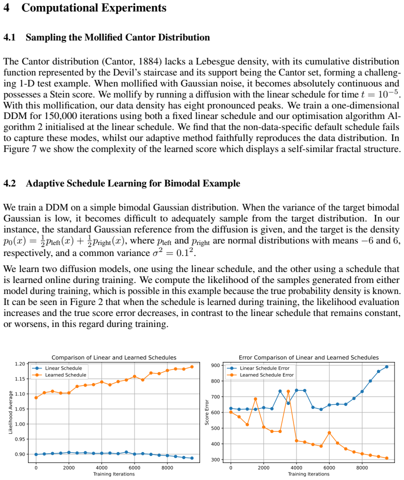
Summary. The paper proposes a principled method for choosing the discretisation schedule used when simulating the reverse diffusion in denoising diffusion models. The authors define an incremental cost L(t,t') based on the work done by a hypothetical predictor-corrector step, derive a local quadratic approximation delta(t) (Theorem 2.1), and then show that, in the dense-schedule limit, the total cost is minimized by the schedule generator phi*(s) = Lambda^{-1}(Lambda s), where Lambda(t) = int_0^t sqrt(delta(u)) du (Theorem 3.1). Algorithm 1 estimates this schedule using score evaluations only, and Algorithm 2 extends it to online training. Experiments on a mollified Cantor distribution, a bimodal example, and CIFAR-10/FFHQ/AFHQv2/ImageNet show that the learned schedules recover the shape of the best hand-tuned Karras schedules and achieve competitive FID scores.
Significance. If the theoretical result is fully established, the paper makes a useful contribution: it gives a parameter-free, data-dependent criterion for schedule selection in diffusion samplers, replacing manual hyperparameter sweeps, and it connects schedule design to a Fisher-divergence geometry of the diffusion path. The proposed cost is derived rather than fit, and the resulting schedule update is cheap and scalable, requiring only score evaluations. The paper also honestly states the main limitations in Section 5: the theory assumes perfect scores and the predictor-corrector formulation, while the image experiments use deterministic Heun solvers with learned scores. The empirical finding that the optimized schedule matches the manually tuned Karras schedule is striking and well presented, although the formal transfer of the optimality theorem to the actual sampler remains an assumption.
major comments (3)
- [Section 2.3, Eq. (14); Appendix A.1] Equation (14) is stated as an exact change of variables, but it is not correct for a general predictor map. With z = F_{t,t'}(x), the pushforward density satisfies q(F(x)) = p_t(x)/|det∇F(x)|, and the correct transformation introduces a factor ∇F^{-T} in the score difference. Consequently the integrand after the change of variables is ||∇F^{-T}∇log G_{t,t'}(x)||^2, not ||∇log G_{t,t'}(x)||^2. This identity is used in the proof of Theorem 2.1 in Appendix A.1, specifically in the mean-value-theorem argument around Eqs. (23)-(26). For the identity predictor the missing factor is harmless, and for the Euler probability-flow predictor of Example 2.2 the discrepancy is O(Δt^3), so the leading-order coefficient δ(t) in Theorem 2.1 is likely correct in the cases used for the main experiments. However, as written, the proof does not establish Theorem 2.1 for arbitrary predictors, and the predictor-optimized cost L_p is therefore not rigorously supported. The authors should either correct Eq. (14) and re-prove Theorem 2.1 directly from Eq. (13), or explicitly state Eq. (14) as an asymptotic leading-order relation and restrict the theorem accordingly.
- [Section 3, Assumption 3.1; Section 4.4] The optimality of φ* is proved under Assumption 3.1, which requires that every predictor-corrector step reaches stationarity, and the paper also assumes perfect score estimation throughout the theoretical derivation. The image experiments in Section 4.4, however, use deterministic second-order Heun/ODE solvers with learned scores and no Langevin corrector, as described in Appendix C.2. Thus Theorem 3.1 does not formally imply that the schedules used in Table 1 minimize FID for these samplers. The authors acknowledge this limitation in Section 5, but the abstract and Section 4.4 state that the method recovers the optimal schedule without this caveat. I recommend that the authors either soften the claim or provide additional empirical evidence that schedules minimizing L_c also minimize the actual sampling error beyond the six-schedule correlation plot in Figure 4 (left).
- [Section 3.1 and Algorithm 1] Theorem 3.1 is a dense-limit statement: as T→∞, T L(φ,T) → E(φ) and L(φ,T) ≳ Λ^2/T. Algorithm 1, however, outputs a finite schedule by interpolating and inverting a finite approximation of Λ. The paper states that for finite T the optimal schedule makes incremental costs approximately constant, but this is only an approximation inherited from the local quadratic expansion. The finite-T schedule produced by the interpolation step is not proved to be the exact minimizer of the finite sum of costs. This is not a fatal issue if presented as an approximation, but the text should distinguish the asymptotic theorem from the finite-T algorithm more carefully.
minor comments (4)
- [Appendix A.1, Eq. (28)] In the expression for log G_{t,t'}(x), the term '- pt(x)' should read '- log p_t(x)'. The printed formula is a typo, but it appears in a proof and should be corrected.
- [Definition 2.2] The type of the corrector is written as L_{t,τ}: X × P(X) → [0,1], which is not the usual notation for a Markov transition kernel. The intended meaning is clear, but the notation is nonstandard and should be cleaned up.
- [Section 4.4 and Table 1] The FID values are reported without error bars or multiple seeds, and the authors justify this in the checklist. This is acceptable practice for this type of experiment, but the paper should explicitly state that the FID differences between the top schedules are within the typical run-to-run variability of a single FID evaluation.
- [Algorithm 1] The monotone spline interpolation used to construct Λ^{-1} is referenced to Fritsch and Carlson (1980), but the implementation details are not given. In particular, the handling of endpoints and the number of quadrature points for the cumulative sums would be useful for reproducibility.
Circularity Check
No significant circularity: the schedule formula is derived from an independently defined cost, and the only self-citation is a non-load-bearing algorithmic adaptation.
full rationale
The paper's central result is a derivation, not a fit: Theorem 2.1 defines the local cost delta(t) from score functions along the diffusion path, and Theorem 3.1 derives phi*(s) = Lambda^{-1}(Lambda s) by minimizing the resulting energy E(phi) through Jensen's inequality. The cost is not defined in terms of the final FID or in terms of the Karras rho=7 schedule, so the empirical agreement in Section 4.4 is independent evidence rather than a forced construction. The only explicit self-citation is 'Algorithm 1 adapts Algorithm 3 from Syed et al. (2021)', but that citation supplies a generic iterative schedule-equalization procedure; it does not carry the proof of optimality, which is established by the paper's own Theorem 3.1 and is supported by the previously published Syed et al. method. The skeptical concern about Eq. (14) omitting a Jacobian-transpose factor is a correctness or rigor issue for general predictors, not a circular reduction: the theorem's conclusion is not assumed among its premises. Likewise, Assumption 3.1 and the perfect-score assumption limit the formal transfer to practical samplers but do not make the derivation circular. Overall, the derivation chain is self-contained apart from a minor, non-load-bearing self-citation.
Assumptions & free parameters
free parameters (2)
- velocity scaling v(t) = sigma(t) =
chosen by hand, not fitted
- schedule learning rate gamma =
0.1 (bimodal/CIFAR), 0.01 (Cantor), 0.05 (MNIST)
assumptions (5)
- domain assumption Perfect score estimation: the cost uses true nabla log p_t
- domain assumption Assumption 3.1: predictor-corrector update yields exact samples from p_{t'}
- standard math Three-times differentiability and domination condition V in Theorem 2.1
- domain assumption Dense-limit approximation L(phi,T) approx E(phi)/T
- domain assumption Langevin corrector dynamics with speed v(t) model the true sampler work
Cite this review
Pith. "Pith review of Score-Optimal Diffusion Schedules." pith.science (2026). https://pith.science/paper/JPVI74LI
@misc{pith2026241207877,
  author       = {Pith},
  title        = {Pith review of: Score-Optimal Diffusion Schedules},
  year         = {2026},
  howpublished = {\url{https://pith.science/paper/JPVI74LI}},
  note         = {Machine review of arXiv:2412.07877}
}
read the original abstract
Denoising diffusion models (DDMs) offer a flexible framework for sampling from high dimensional data distributions. DDMs generate a path of probability distributions interpolating between a reference Gaussian distribution and a data distribution by incrementally injecting noise into the data. To numerically simulate the sampling process, a discretisation schedule from the reference back towards clean data must be chosen. An appropriate discretisation schedule is crucial to obtain high quality samples. However, beyond hand crafted heuristics, a general method for choosing this schedule remains elusive. This paper presents a novel algorithm for adaptively selecting an optimal discretisation schedule with respect to a cost that we derive. Our cost measures the work done by the simulation procedure to transport samples from one point in the diffusion path to the next. Our method does not require hyperparameter tuning and adapts to the dynamics and geometry of the diffusion path. Our algorithm only involves the evaluation of the estimated Stein score, making it scalable to existing pre-trained models at inference time and online during training. We find that our learned schedule recovers performant schedules previously only discovered through manual search and obtains competitive FID scores on image datasets.
Figures


Figures from the paper (10 more)


Forward citations
Cited by 2 Pith papers
-
Optimal Scheduling of Dynamic Transport
For a fixed transport map with symmetric positive definite Jacobian, the closed-form optimal schedule minimizing the uniform spatial Lipschitz constant of the flow velocity is an exponential two-phase curve that achie...
-
A Fourier Space Perspective on Diffusion Models
EqualSNR, a diffusion forward process that corrupts every Fourier frequency at the same rate, improves high-frequency generation quality while matching DDPM's FID on standard image benchmarks.
Reference graph
Works this paper leans on
-
[1]
Claims Question: Do the main claims made in the abstract and introduction accurately reflect the paper’s contributions and scope? Answer: [Yes] . Justification: Our main theoretical and experimental contributions are clearly stated in the abstract and demonstrated in the paper. They reflect the paper’s contributions and scope
-
[2]
Limitations Question: Does the paper discuss the limitations of the work performed by the authors? Answer: [Yes] Justification: We discuss the limitations of our work in Section 5
-
[3]
Justification: All the proofs are proven in the supplementary material
Theory Assumptions and Proofs Question: For each theoretical result, does the paper provide the full set of assumptions and a complete (and correct) proof? Answer: [Yes] . Justification: All the proofs are proven in the supplementary material. They are duly cross-referenced
-
[4]
Experimental Result Reproducibility Question: Does the paper fully disclose all the information needed to reproduce the main ex- perimental results of the paper to the extent that it affects the main claims and/or conclusions of the paper (regardless of whether the code and data are provided or not)? Answer: [Yes] Justification: We provide detailed descri...
-
[5]
Open access to data and code Question: Does the paper provide open access to the data and code, with sufficient instruc- tions to faithfully reproduce the main experimental results, as described in supplemental material? Answer: [Yes] Justification: We provide the code necessary to run our experiments
-
[6]
Experimental Setting/Details Question: Does the paper specify all the training and test details (e.g., data splits, hyper- parameters, how they were chosen, type of optimizer, etc.) necessary to understand the results? Answer: [Yes] Justification: We provide all our experiment details in Appendix C
-
[7]
Standard deviations could be bootstrapped from this set but this is not standard practice
Experiment Statistical Significance Question: Does the paper report error bars suitably and correctly defined or other appropriate information about the statistical significance of the experiments? Answer: [No] Justification: Our main metric is FID score for which it is standard practice to report it calculated on the first 50,000 images generated from th...
-
[8]
Experiments Compute Resources Question: For each experiment, does the paper provide sufficient information on the com- puter resources (type of compute workers, memory, time of execution) needed to reproduce the experiments? 23 Answer: [Yes] Justification: We provide details of the compute resources used in Appendix C
Show all 15 references
-
[9]
Justification: After careful review of the NeurIPS Code of Ethics, it is clear that the research presented in this paper conforms with the Code of Ethics in every respect
Code Of Ethics Question: Does the research conducted in the paper conform, in every respect, with the NeurIPS Code of Ethics https://neurips.cc/public/EthicsGuidelines? Answer: [Yes] . Justification: After careful review of the NeurIPS Code of Ethics, it is clear that the rese...
-
[10]
Justification: This paper is mostly theoretical and methodological
Broader Impacts Question: Does the paper discuss both potential positive societal impacts and negative societal impacts of the work performed? Answer: [NA] . Justification: This paper is mostly theoretical and methodological. We do not see immediate societal impact of this wor...
-
[11]
Justification: The paper poses no such risks
Safeguards Question: Does the paper describe safeguards that have been put in place for responsible release of data or models that have a high risk for misuse (e.g., pretrained language models, image generators, or scraped datasets)? Answer: [NA] . Justification: The paper pos...
-
[12]
Licenses for existing assets Question: Are the creators or original owners of assets (e.g., code, data, models), used in the paper, properly credited and are the license and terms of use explicitly mentioned and properly respected? Answer: [Yes] Justification: We provide the r...
-
[13]
Guidelines:
New Assets Question: Are new assets introduced in the paper well documented and is the documentation provided alongside the assets? Answer: [NA] Justification: This paper does not introduce any new assets. Guidelines:
-
[14]
Justification: The paper does not involve crowdsourcing nor research with human subjects
Crowdsourcing and Research with Human Subjects Question: For crowdsourcing experiments and research with human subjects, does the paper include the full text of instructions given to participants and screenshots, if applicable, as well as details about compensation (if any)? A...
-
[15]
Justification: The paper does not involve crowdsourcing nor research with human subjects
Institutional Review Board (IRB) Approvals or Equivalent for Research with Human Subjects Question: Does the paper describe potential risks incurred by study participants, whether such risks were disclosed to the subjects, and whether Institutional Review Board (IRB) approvals...
Reviewed August 11, 2026 · model on record in the stance chip above.
Discussion (0). Continue with ORCID to comment.