REVIEW 5 major objections 6 minor 23 references
Numerical Solution Partial Differential Equations using the Discrete Fourier Transform
T0 review · 5 major / 6 minor · reviewed 2026-08-11 · deepseek-v4-flash
Pith's one-line read The paper shows that the Fast Fourier Transform can numerically solve the Poisson, diffusion, and wave equations in two dimensions by turning spatial derivatives into algebraic factors and time evolution into per-mode ODEs.
desk verdict A standard FFT spectral method tutorial with no new research content; useful for students once the missing periodicity assumption and sign-consistency typos are fixed. read the letter →
The pith
A machine-rendered reading of the paper's core claim, the machinery that carries it, and where it could break.
The reading
What carries the argument
The central object is the discrete Fourier transform (DFT), written as $\vec{P}=W\vec{p}$ with $W_{jk}=\omega_N^{jk}$ and $\omega_N=e^{2\pi i/N}$, together with its inverse $W^{-1}=\frac{1}{N}W^\dagger$. The property that carries the argument is the differentiation rule $\mathcal{F}\{\partial^k u/\partial x^k\}=(-i\omega)^k\mathcal{F}\{u\}$, which converts spatial derivatives into algebraic factors in frequency space. The paper's recipe is to apply the fast version of this transform (FFT) to the equation and initial data, solve the resulting algebraic equations or decoupled ODEs mode by mode, and invert the transform to recover the solution.
What would settle it
Compare the paper's FFT solution of the Poisson equation with a manufactured non-periodic exact solution, for instance $u(x,y)=\sin(\pi x)\sin(\pi y)$ on $[0,1]^2$ with source $s=-2\pi^2 u$: the DFT's implicit periodicity makes the numerical solution disagree with the exact one near the boundary. A periodic exact solution, by contrast, would be recovered to machine precision, showing that the periodic-boundary assumption is what the method's validity rests on.
Extended reading notes
Core claim
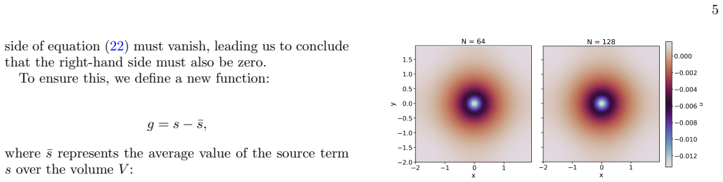
The central claim is that the FFT, applied in the way the paper describes, produces reliable numerical solutions for elliptic, parabolic, and hyperbolic PDEs on discrete two-dimensional domains. For the Poisson equation the Laplace operator becomes multiplication by $-\omega^2$ in frequency space; for the diffusion equation each Fourier mode evolves independently via an exponential decay factor; for the wave equation the transformed problem is a family of forced harmonic oscillators. The paper illustrates each case with concrete numerical examples, including a Gaussian source for Poisson, a Gaussian initial profile for diffusion, and both source-free and orbiting-source cases for the wave equation. It also reports that the spatial average is conserved to within $10^{-12}$ in the evolution examples and that the RK4 solutions self-converge with the expected factor $2^4$, evidence that the recipe works as stated.
Load-bearing premise
The recipe treats the computational domain as periodic because the DFT is periodic, and the paper states this assumption only for the wave equation, not for the Poisson or diffusion examples.
Editorial extensions
If this is right
- For the diffusion equation with zero source, each Fourier mode evolves as $\hat{f}e^{-\omega^2 t}$, so the FFT method reproduces both dissipation and conservation of the spatial average, with $\bar{u}/\bar{f}=1$ to numerical precision.
- For a time-independent source, the wave equation's frequency-space solution is the closed form in equations (36) and (37), so no time integrator is needed; the paper uses these formulas for the source-free example.
- When the source depends on time, the transformed wave equation becomes a system of forced harmonic oscillators that can be integrated with a standard Runge-Kutta method; the paper demonstrates RK4 and verifies the expected fourth-order self-convergence factor $2^4$.
- Because the DFT is periodic, every solution produced by this recipe is the solution on a periodic domain; the paper states this for the wave equation and illustrates the resulting re-entry of wavefronts through the opposite boundary.
- The tutorial is positioned as a starting point for students to move to coupled systems such as Schr\"odinger-Poisson and Bose-Einstein condensate simulations, where the same FFT-based spectral approach is used.
Reading between the lines
- Beyond the paper, the same diagonalization argument shows that for non-periodic boundary conditions the DFT must be replaced by a basis that respects those boundaries, such as a sine or Chebyshev transform; the paper's recipe would otherwise introduce boundary errors.
- A test the paper does not run is to compare the Poisson solution against a manufactured exact solution at several grid sizes and plot the error versus $N$, which would show the spatial convergence rate directly rather than only consistency between two resolutions.
- The zero-frequency mode that the paper shows conserving $\bar{u}$ is the same mechanism by which FFT-based Schr\"odinger-Poisson and Bose-Einstein condensate solvers conserve total mass; the paper mentions these applications as motivation but does not draw this connection.
Editorial analysis
A structured set of objections, weighed in public.
Referee Report
Summary. This manuscript is a pedagogical tutorial on using the DFT/FFT for partial differential equations. It introduces the sampling theorem, defines the DFT in one and two dimensions, sketches the FFT decomposition, and then applies the method to three two-dimensional examples: the Poisson equation, the diffusion equation, and the wave equation. The paper is descriptive rather than analytical, uses Gaussian profiles on square domains, and claims to give students a reliable starting point for applying FFT methods to more advanced problems.
Significance. If the technical issues are corrected, this would be a useful tutorial for a physics education venue: it covers elliptic, parabolic, and hyperbolic equations, discusses aliasing and computational complexity, and includes conservation and self-convergence checks. The method itself is standard spectral theory, so the value is pedagogical rather than novel. The paper does not include machine-checked proofs or reproducible code, but it does present concrete numbered equations and figures that a student could re-implement after the notation is fixed. The main weaknesses are an unstated periodicity requirement for two of the three examples, an internally inconsistent DFT sign convention, and a wrong exact-solution formula for the forced wave equation.
major comments (5)
- [Section III.A; Section III.B] Neither the Poisson example (III.A) nor the diffusion example (III.B) states the boundary condition under which the DFT solution is computed, although a DFT on a finite uniform grid represents the periodic extension of the data. The wave-equation section explicitly says that boundary conditions for problem (32)-(33) will be assumed periodic, but the parallel statement is absent for Eq. (21) and Eqs. (27)-(28). Consequently, Eq. (25) and Eq. (30) produce toroidal (periodic) solutions, not solutions of ordinary Dirichlet or Neumann boundary-value problems. The Gaussian source and initial data decay at the boundary and therefore mask the issue, but a student reusing the same recipe on a non-periodic problem will silently obtain a wrong solution. The revision should state the periodic-domain assumption in all three examples and explain its practical meaning.
- [Section III.C, Eq. (37)] The exact solution of the forced oscillator in Eq. (37) is incorrect: it omits the particular solution \hat{s}/\omega^2. The correct expression for a time-independent source is \hat{u}(t)=(\hat{f}-\hat{s}/\omega^2)\cos(\omega t)+(\hat{g}/\omega)\sin(\omega t)+\hat{s}/\omega^2. As printed, Eq. (37) does not satisfy d^2\hat{u}/dt^2+\omega^2\hat{u}=\hat{s}. The error is not visible in the s=0 example that follows, but the text presents Eq. (37) as a general exact solution for time-independent sources.
- [Section II.D, Eqs. (17) and (19)-(20)] The definition of the two-dimensional DFT is internally inconsistent. Equation (17) uses e^{+2\pi i a j/N_x} e^{+2\pi i b k/N_y}, while the row-by-row factorization in Eqs. (19) and (20) uses e^{-2\pi i a j/N_x} and e^{-2\pi i b k/N_y}. These signs correspond to opposite transform conventions. Since the transformed PDEs in Section III depend on the sign convention through the algebraic representation of derivatives, the paper must choose a single convention, preferably the one used by the FFT implementation a student would call, and apply it consistently in all equations.
- [Section III.B, Eq. (30); Section II.D] The transition from the continuous frequency variable \omega to the discrete DFT indices is never specified for the two-dimensional examples. Equations (29), (30), (34), (36), and (37) use \omega^2 as a scalar, but on a two-dimensional grid \omega is a wave vector whose components are related to k_x^a and k_y^b in Eq. (18). The paper should state, for example, that \omega^2=(2\pi k_x^a)^2+(2\pi k_y^b)^2 with the chosen sign convention, and it should explain how the factor 2\pi and the zero mode are handled. Without this mapping the recipe cannot be implemented from the text alone.
- [Section III.C.2, Eq. (39)] The self-convergence test is used to conclude that the solutions are 'self-convergent, in one word, numerically correct.' The ratio in Eq. (39) only verifies that differences between three resolutions follow the expected 16:1 scaling of the RK4 method; it does not verify that the discrete solution satisfies the intended PDE, boundary conditions, or sign convention, because those errors can also be self-convergent. For the s=0 wave example an exact solution is available and should be used for a direct error comparison. For the orbiting-source example, the claim should be softened to a necessary consistency check rather than a proof of correctness.
minor comments (6)
- [Eq. (4)] The Riemann-sum error is stated as O(\Delta t^2), but a simple left Riemann sum has first-order error O(\Delta t); if the trapezoidal rule is intended, that should be stated explicitly.
- [Eq. (30)] The special branch for \omega=0 in Eq. (30) is redundant, because \hat{f} e^{-\omega^2 t}=\hat{f} also holds at \omega=0; the distinction may confuse readers.
- [Section III.A] After the mean subtraction in Eqs. (23)-(24), the zero-frequency component of \hat{g} vanishes, but Eq. (25) still contains a division by \omega^2; the paper should state explicitly that the k=0 component of the computed quotient is set to zero, which also fixes the arbitrary additive constant of the Poisson solution.
- [Section III.C.2] For the time-dependent orbiting source, the paper does not explain how \hat{s}(t) is obtained at intermediate RK4 stages; a sentence stating that the FFT of s(t,x,y) is recomputed at each stage would make the algorithm reproducible.
- [General] There are several typographical errors: 'Hyperpolic' in the Section III.C heading, 'Dissipation' for the diffusion equation in the Introduction, 'aself-convergence' before Eq. (39), 'Foe' before Eq. (22), and 'tw-dimensional' in Section II.D.
- [Abstract/PACS line] The line 'PACS numbers: keywords: Partial Differential Equations ...' is garbled; PACS codes and keywords should be listed as separate metadata fields.
Circularity Check
No significant circularity: the FFT-based PDE solutions follow from standard Fourier identities with no fitted parameters, and the only self-citations are motivational.
full rationale
The paper's derivation chain is self-contained with respect to its central numerical recipe. The Poisson solution in Eq. (25) is obtained by applying the Fourier differentiation property to Eq. (21)-(22), solving algebraically for F{u}, and then inverse-transforming; no parameter is fitted to any computed solution. The diffusion solution in Eq. (30) is the closed-form integration of the decoupled ODEs in Eq. (29), again with no free parameters calibrated to output data. The wave-equation solutions in Eqs. (36)-(37) are exact solutions of the forced-oscillator ODEs derived in Eq. (35) from the Fourier-transformed wave equation. These are standard Fourier identities applied directly, and the paper does not rename a known empirical pattern nor import a uniqueness theorem. The self-citations to the authors' prior work ([12] and [14]) appear only in the final motivational remarks about Schrödinger-Poisson systems and quantum computing; they do not support any load-bearing step of the method. The skeptical concern about unstated periodic boundary conditions for the Poisson and diffusion examples is a legitimate correctness/scope gap, but it is not circularity: the derivation does not assume its conclusion. Similarly, the sign inconsistency between Eqs. (17) and (19)-(20) is a typographical/reproducibility issue, not a circular reduction. Thus the appropriate circularity score is 0.
Assumptions & free parameters
assumptions (4)
- domain assumption The DFT of a periodic sample represents the function's Fourier coefficients on a periodic domain.
- domain assumption The source function and solution are regular enough for the Fourier transform of the Laplacian to be -omega^2 times the transform.
- standard math Sampling theorem and Nyquist frequency determine aliasing limits.
- standard math DFT orthogonality gives a unique invertible transform.
Cite this review
Pith. "Pith review of Numerical Solution Partial Differential Equations using the Discrete Fourier Transform." pith.science (2026). https://pith.science/paper/EI6TYV4F
@misc{pith2026241212308,
  author       = {Pith},
  title        = {Pith review of: Numerical Solution Partial Differential Equations using the Discrete Fourier Transform},
  year         = {2026},
  howpublished = {\url{https://pith.science/paper/EI6TYV4F}},
  note         = {Machine review of arXiv:2412.12308}
}
read the original abstract
In this paper we explain how to use the Fast Fourier Transform (FFT) to solve partial differential equations (PDEs). We start by defining appropriate discrete domains in coordinate and frequency domains. Then describe the main limitation of the method arising from the Sampling Theorem, which defines the critical Nyquist frequency and the aliasing effect. We then define the Fourier Transform (FT) and the FFT in a way that can be implemented in one and more dimensions. Finally, we show how to apply the FFT in the solution of PDEs related to problems involving two spatial dimensions, specifically the Poisson equation, the diffusion equation and the wave equation for elliptic, parabolic and hyperbolic cases respectively.
Figures


Figures from the paper (6 more)


Reference graph
Works this paper leans on
-
[1]
The DFT is periodic, i.e., Pk+N = Pk
-
[2]
The inverse of the matrix W is given by W−1 = 1 N W†, where W† is the conjugate transpose of W. The second property allows us to recover the original function from its Fourier components via the inverse DFT (iDF T) given by: pj = 1 N N −1X k=0 Pkω−jk N , (10) 3 FIG. 1. Left: Approximation of the FT in the original fre- quency domain. Right: The same signa...
work page 2000
-
[3]
Example with s = 0. The problem is to solve the wave equation for an initial time-symmetric spherically symmetric Gaussian pulse in the domain D = [−1, 1]2. The set up of the problem is then with s = 0 and initial conditions f (x, y) = Ae−(x2+y2)/σ2 g(x, y) = 0 . in the discrete domain that uses N = 128, to be inte- grated in the time domain t ∈ [0, 2]. I...
-
[4]
Example with Source Another typical solution of the wave equation involves a source that orbits the origin on the xy-plane, leaving behind a strip. The source is given by: s(t, x, y) = Ae−[(x−x0)2+(y−y0)2]/σ2 s cos(γt), (38) where the center of the source ( x0, y0) orbits in a cir- cle of radius rs, described by x0 = rs cos(Ωt) and y0 = rs sin(Ωt). In thi...
-
[5]
Revisiting spherically symmetric relativistic hydrody- namics,
F. S. Guzm´ an, F. D. Lora-Clavijo, and M. D. Morales, “Revisiting spherically symmetric relativistic hydrody- namics,” Revista Mexicana de Fisica E 58, 84–98 (2012)
work page 2012
-
[6]
F. S. Guzm´ an,Numerical Methods for Initial Value Prob- lems in Physics , Springer, Switzerland No. v. 1 (Springer, 2023)
work page 2023
-
[7]
Solving the time-dependent schroedinger equation using finite difference methods,
R. Becerril, F.S. Guzman, A. Rendon-Romero, and S. Valdez-Alvarado, “Solving the time-dependent schroedinger equation using finite difference methods,” Revista Mexicana de Fisica E 54, 120–132 (2008)
work page 2008
-
[8]
F.S. Guzm´ an, “Soluci´ on de la ecuaci´ on de onda como un problema de valores iniciales usando diferencias finitas,” Revista Mexicana de Fisica E 56, 51 (2010)
work page 2010
Show all 23 references
-
[9]
Pseudospectral vs finite differences methods in numer- ical relativity,
I Avil´ es, G. Estrada, J. A Gonz´ alez, and F. S. Guzm´ an, “Pseudospectral vs finite differences methods in numer- ical relativity,” Revista Mexicana de Fisica E 63, 25–32 (2017)
2017
-
[10]
William H Press, Brian P Flannery, Saul A Teukolsky, and William T Vetterling, Numerical Recipes: The Art of Scientific Computing (Cambridge University Press, 1986)
1986
-
[11]
Exact solution of the 1d shock-tube problem in newtonian and relativistic hydrodynamics,
F. D. Lora-Clavijo, J. P. Cruz-P´ erez, F. S. Guzm´ an, and J. A. Gonz´ alez, “Exact solution of the 1d shock-tube problem in newtonian and relativistic hydrodynamics,” Revista Mexicana de Fisica E 59, 28–50 (2013)
2013
-
[12]
Spherical accretion of a perfect fluid onto a black hole,
F. S. Guzm´ an, A. Romero-Amezcua, and I. ´Alvarez- R ´ ıos, “Spherical accretion of a perfect fluid onto a black hole,” Revista Mexicana de Fisica E 59, 020206 (2021)
2021
-
[13]
An algorithm for the machine calculation of complex fourier series,
James W. Cooley and John W. Tukey, “An algorithm for the machine calculation of complex fourier series,” Mathematics of Computation 19, 297–301 (1965)
1965
-
[14]
Spiegel, Schaum’s Outline of Fourier Analysis with Applications to Boundary Value Problems , Schaum’s Outline Series (McGraw Hill LLC, 1974)
M.R. Spiegel, Schaum’s Outline of Fourier Analysis with Applications to Boundary Value Problems , Schaum’s Outline Series (McGraw Hill LLC, 1974)
1974
-
[15]
A Living Review of Quantum Computing for Plasma Physics,
´Oscar Amaro and Diogo Cruz, “A Living Review of Quantum Computing for Plasma Physics,” arXiv e-prints , arXiv:2302.00001 (2023), arXiv:2302.00001 [physics.plasm-ph]
2023 arXiv
-
[16]
Galaxy formation with BECDM I. Turbulence and relaxation of idealized haloes,
Philip Mocz, Mark Vogelsberger, Victor H. Robles, Jesus Zavala, Michael Boylan-Kolchin, Anastasia Fi- alkov, and Lars Hernquist, “Galaxy formation with BECDM I. Turbulence and relaxation of idealized haloes,” Mon. Not. Roy. Astron. Soc. 471, 4559–4570 (2017), arXiv:1705.05845 ...
2017 arXiv
-
[17]
Explo- ration of simple scenarios involving fuzzy dark matter cores and gas at local scales,
Iv´ an ´Alvarez-Rios and Francisco S Guzm´ an, “Explo- ration of simple scenarios involving fuzzy dark matter cores and gas at local scales,” Monthly Notices of the Royal Astronomical Society 518, 3838–3849 (2022)
2022
-
[18]
Mathematical theory and numerical methods for bose-einstein condensation,
Weizhu Bao and Yongyong Cai, “Mathematical theory and numerical methods for bose-einstein condensation,” Kinetic and Related Models 6, 1–135 (2013)
2013
-
[19]
Variational quantum crank-nicolson and method-of- lines schemes for the solution of initial value problems,
Francisco Guzman-Cajica and Francisco S. Guzm´ an, “Variational quantum crank-nicolson and method-of- lines schemes for the solution of initial value problems,” Phys. Rev. A 110, 042415 (2024)
2024
-
[21]
Application of a variational hybrid quantum-classical algorithm to heat conduction equation and analysis of time complexity,
Y. Y. Liu, Z. Chen, C. Shu, S. C. Chew, B. C. Khoo, X. Zhao, and Y. D. Cui, “Application of a variational hybrid quantum-classical algorithm to heat conduction equation and analysis of time complexity,” Physics of Fluids 34, 117121 (2022), arXiv:2207.14630 [quant-ph]
2022 arXiv
-
[22]
Variational Quantum Evolution Equa- tion Solver,
Fong Yew Leong, Wei-Bin Ewe, and Dax En- shan Koh, “Variational Quantum Evolution Equa- tion Solver,” arXiv e-prints , arXiv:2204.02912 (2022), arXiv:2204.02912 [quant-ph]
2022 arXiv
-
[23]
Quantum Variational Solving of Nonlinear and Multi-Dimensional Partial Dif- ferential Equations,
Abhijat Sarma, Thomas W. Watts, Mudassir Moosa, Yil- ian Liu, and Peter L. McMahon, “Quantum Variational Solving of Nonlinear and Multi-Dimensional Partial Dif- ferential Equations,” arXiv e-prints , arXiv:2311.01531 (2023), arXiv:2311.01531 [quant-ph]
2023 arXiv
-
[256]
Vari- ous snapshots of the solution, obtained using the Runge- Kutta 4 (RK4) scheme to integrate Eq
The temporal resolution is set to ∆ t = 0.25h. Vari- ous snapshots of the solution, obtained using the Runge- Kutta 4 (RK4) scheme to integrate Eq. (35), are shown in Figure 8. 8 FIG. 7. Normalized average value of the function u over time, relative to the initial average ¯f ....
2024
Reviewed August 11, 2026 · model on record in the stance chip above.
Discussion (0). Continue with ORCID to comment.