REVIEW 3 major objections 6 minor 35 references
Microscopic imprints of learned solutions in adaptive resistor networks
T0 review · 3 major / 6 minor · reviewed 2026-08-11 · deepseek-v4-flash
Pith's one-line read A trained resistor network leaves its whole learned task imprinted in one experimentally measurable susceptibility tensor.
desk verdict Clean math, under-supported empirics, worth peer review with a request for finite-cost bounds. read the letter →
The pith
A machine-rendered reading of the paper's core claim, the machinery that carries it, and where it could break.
The reading
What carries the argument
The load-bearing object is the per-edge susceptibility vector $s_i = \bar{\Delta}_i^T H^{-1}$, where $\bar{\Delta}_i$ is the extended incidence row of edge $i$ and $H$ is the extended physical Hessian (bordered Laplacian) of the grounded resistor network. Its entries are voltage drops across edge $i$ induced by unit currents at each node, and its squared norm is a scalar susceptibility per edge. The identity $S_{ij} = 4\,s_i \otimes s_i \otimes s_j \otimes s_j$ reduces the entire susceptibility tensor to these vectors, after the derivative $\partial H^{-1}/\partial k_i = -2\,s_i \otimes s_i$ is computed from the matrix-inverse rule. Because $\|s_i\|^2 = \sum_\alpha \nu_\alpha^{-2}(\bar{\Delta}_i^T W_\alpha)^2$, the susceptibility is dominated by soft modes, which is what ties it to low-dimensional responses and to the stiff modes of the cost Hessian.
What would settle it
Simulate training on one fixed regression task but stop at a ladder of final costs from $C\approx10^{-9}$ to $C\approx1$; compute each network's susceptibility norms and the stiff modes of the true cost Hessian, and plot their correlation versus $C$. If the correlation collapses well before the costs reached in realistic training, then susceptibility carries the relevant physical information only at the idealized zero-cost point, not for trained networks as realized.
Extended reading notes
Core claim
The paper's central claim is an exact factorization of the cost Hessian for a successfully trained physical network: $\mathcal{H}_{ij} = \mathcal{L}\,\cdots\,S_{ij}$ (full contraction), where $\mathcal{L}$ is a fourth-rank training tensor built only from the input currents and output projectors, and the susceptibility tensor is $S_{ij} = 4\,s_i \otimes s_i \otimes s_j \otimes s_j$, with $s_i = \bar{\Delta}_i^T H^{-1}$ the susceptibility vector of edge $i$. Each component of $s_i$ is the voltage drop across edge $i$ when a unit current is injected at one node, so the whole tensor is a linear-response observable. The paper shows numerically that the norm $\|s_i\|^2$ is dominated by the softest modes of the physical Hessian and that, across linear regression (two and five outputs), three-class classification, and allosteric edge tasks, highly susceptible edges coincide with the entries of the stiff eigenmodes of the cost Hessian. It further shows that these edges have low relative conductance and act as current-blocking walls or corridors, and it argues that the same derivation applies to any physical network whose response minimizes a Lyapunov function, with all physical information captured up to quadratic order in the physical landscape.
Load-bearing premise
The entire derivation assumes the trained network has cost exactly zero, meaning every task constraint is satisfied perfectly; the simulations only reach small nonzero costs ($C\approx10^{-5}$ to $10^{-9}$, and $C\approx0.05$ for classification), and no bound is given for how the susceptibility-importance correlation behaves as the cost grows.
Editorial extensions
If this is right
- Key functional edges can be identified from physics alone: measuring voltage responses to unit currents gives $s_i$, and high-susceptibility edges are the ones whose perturbation hurts the trained task most.
- The same susceptibility measurement works without knowing the task specification, so trained networks become interpretable in an experimentally non-invasive way.
- Because the factorization is independent of the training protocol, it applies to any route to a zero-cost solution, including local learning rules, global optimization, and evolutionary or biological processes.
- Previously observed phenomena: low-dimensional physical response, stiff-mode/soft-mode correspondence, and topological sector structure in allosteric networks, follow as corollaries of the susceptibility tensor.
- For nonlinear physical networks, all physical information up to quadratic order in the physical landscape is still contained in the susceptibility tensor.
Reading between the lines
- A natural test the paper leaves open is the finite-cost regime: measuring how the susceptibility-to-stiff-mode correlation degrades as the final cost rises from $10^{-9}$ to $O(1)$ would map the practical validity of the exact factorization.
- The wall-and-corridor picture suggests a design heuristic not stated in the paper: placing low-conductance barriers along high-susceptibility edges before training may bias learning toward solutions that are easier to interpret and possibly more robust.
- By analogy to the allosteric discussion, a susceptibility-like response matrix could serve as an experimental probe of global epistasis in proteins, connecting slow physical modes to non-additive mutation effects without needing the task to be a single-mode response.
- Because the susceptibility is a property of the physical Hessian alone, one could compute it in untrained networks as well; if high-susceptibility edges are also enriched in networks that train faster, the quantity would double as a trainability predictor.
Signed reviews
Editorial analysis
A structured set of objections, weighed in public.
Referee Report
Summary. The paper studies trained adaptive resistor networks and derives an exact factorization of the cost Hessian at the learned solution. In Section III, under the assumption that all task constraints are satisfied exactly (C=0), the cost Hessian is written as a contraction of a task-dependent training tensor L and a physical susceptibility tensor S. Section IV simplifies the susceptibility tensor to products of per-edge susceptibility vectors si = Δ^T_i H^{-1}, where H is the physical (bordered Laplacian) Hessian, and shows that susceptibility norms are dominated by soft physical modes. The paper then presents numerical correlations between susceptibility and stiff cost modes for linear regression, classification, and allosteric tasks, and interprets highly susceptible edges as current-blocking 'walls' or 'corridors' that implement the learned function. The authors argue that susceptibility provides a task-agnostic, experimentally measurable probe of learned functionality.
Significance. The algebraic core of the paper is elegant and, as far as I can verify, correct: differentiating H^{-1} gives -2 si⊗si, and the contraction in Eq. (12) follows from the chain rule. If the finite-cost and correlation issues are resolved, this factorization usefully unifies earlier observations about low-dimensional physical responses, stiff-mode correspondence, and topological sectors under a single susceptibility-based framework. The proposed quantity is experimentally accessible and independent of the training protocol, which is a genuine strength. However, the demonstrated support for the central 'susceptibility captures functional importance' claim is currently qualitative, and the exactness of the factorization is tied to a zero-cost limit that the simulations only approximately reach. The paper therefore has solid potential but needs strengthening of the demonstrative layer before its claims are fully supported.
major comments (3)
- [III (Eq. (7), Assumption I) and Appendix D] The exact factorization in Eq. (12) is derived under Assumption I (cr=0 for every task), which eliminates the second-derivative term from the cost Hessian. The simulations in Appendix D reach finite costs: C≈10^-5, 10^-8, and 1×10^-5 for the regression and allosteric tasks, but C≈0.05 for the cosine-similarity classification cost of Eq. (23). For the classification example, ||cr|| ~ sqrt(C) ~ 0.2, so the omitted term Σ_r c_r^T ∂²c_r/∂k_i∂k_j can be comparable to the retained first-derivative term. The paper does not bound this correction or show empirically that the C=0 factorization remains accurate at C=0.05. Please quantify the correction (for instance, by comparing the exact cost Hessian with the factorization on a trained network) or explicitly qualify the central claim as holding only in the C→0 limit.
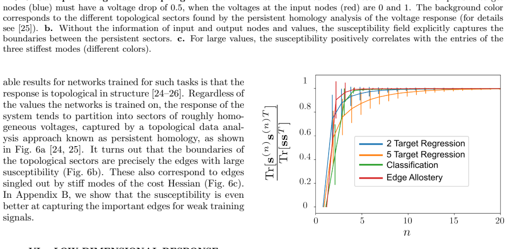
- [V, Figs. 4d, 5d, 5h, 6c] The claim that edge susceptibility 'correlates positively' with stiff-mode entries is supported only by scatter plots. No correlation coefficient, confidence interval, or significance test is reported, and the ensemble of 50 initial conditions used in Fig. 7 is not used to assess the variability of the claimed correlations across tasks. Please report quantitative correlation measures (for example, Spearman rank correlation with bootstrap uncertainties) for each task, together with the number of edges used in each comparison. This is necessary to judge the strength of the demonstrated correspondence and to support the abstract's unqualified statement that susceptibility 'captures' the relevant physical information.
- [VIII and Abstract] The abstract and Discussion state that 'all the physical information relevant to the trained input-output relation can be captured by a susceptibility.' This statement is exact only at C=0 and for responses that are linear perturbations around a local minimum (conditions II and III in Section IV). For nonlinear networks, the factorization holds only to quadratic order in the physical landscape, as acknowledged in Eq. (21) and the surrounding text. Please qualify the scope of the claim in the abstract and Discussion, particularly because one of the demonstrated examples (classification) operates at a finite cost where the exact identity does not hold.
minor comments (6)
- [II and III (Eqs. (2) and (7))] The physical Hessian is denoted H in Eq. (2) and the cost Hessian is also denoted H in Eq. (7); please use distinct symbols (e.g., H^phys and H^cost) or consistent boldface to avoid confusion.
- [IV] The sentence 'we obtain Sij∼H^{-4}, and ultimately H∼H^{-4}' uses the same symbol H for both the susceptibility tensor and the cost Hessian; please disambiguate the notation.
- [Fig. 7 caption] The caption refers to 'full susceptibility' without defining it; please define it as s_i^{(N+1)} and state that n is the number of modes retained in Eq. (24).
- [Throughout] Figure references are inconsistent in capitalization ('fig.', 'Fig.', 'Figure'); please standardize to a single style.
- [Appendix B] The text says that susceptibility is 'even better at capturing the important edges for weak training signals,' but Fig. 12 appears only to show overlap with the single stiff mode; please clarify what 'better' is compared with (e.g., persistent homology sectors) and define the metric used for the comparison.
- [References] Reference [15] is cited as an arXiv preprint; please update it if a journal version has appeared, and check that all references contain complete publication data.
Circularity Check
No significant circularity: the cost-Hessian factorization is a derived algebraic identity, re-derived in Appendix A, and checked against independently computed cost-Hessian eigenvectors; the finite-cost caveat is a correctness risk, not circularity.
full rationale
The paper's central result is the identity H_ij = L....S_ij (Eq. 12) with S_ij = 4 s_i⊗s_i⊗s_j⊗s_j (Eq. 16), obtained from the chain rule applied to V_F = H^{-1}I (Eq. 4) and the C=0 cost Hessian (Eq. 7). This is an algebraic derivation, not a fitted or assumed relation. The susceptibility vectors s_i are defined directly from the physical Hessian and are computed, not tuned, in the simulations; the correlation between susceptibility and stiff modes of the cost Hessian is benchmarked against independently computed eigenvectors (Figs. 4d, 5d, 5h, 6c). The only self-citation for Eq. (7) is to Ref. [15], but the same formula is re-derived for general differentiable costs in Appendix A (Eqs. A1–A7), so the citation is not load-bearing. The derivation explicitly assumes C=0 (Assumption I, Section III), while simulations reach small but nonzero costs (C ~ 10^-5 to 10^-9, and C ~ 0.05 for classification). The unquantified finite-cost correction is a stated limitation and a correctness risk, not a circular step: the paper neither hides the assumption nor redefines the correction as a prediction. No fitted parameter is renamed as a prediction, and no uniqueness theorem or ansatz is imported from the authors' prior work to force the conclusion. The derivation chain is therefore self-contained; the observed correlations are nontrivial numerical checks rather than consequences of the definitions alone.
Assumptions & free parameters
assumptions (4)
- domain assumption The physical response minimizes dissipated power P(V,I) at fixed conductances (Kirchhoff's current law), so VF = H^{-1} I.
- domain assumption Training reaches a global minimum with all constraints satisfied exactly, cr=0 for all tasks.
- domain assumption The response is well approximated by a linear perturbation around a known local minimum for nonlinear generalizations, VF ≈ Vmin + H^{-1} I.
- standard math The bordered physical Hessian H is invertible after grounding, and its eigenvectors are orthonormal.
Cite this review
Pith. "Pith review of Microscopic imprints of learned solutions in adaptive resistor networks." pith.science (2026). https://pith.science/paper/I6UPI5RU
@misc{pith2026241219356,
  author       = {Pith},
  title        = {Pith review of: Microscopic imprints of learned solutions in adaptive resistor networks},
  year         = {2026},
  howpublished = {\url{https://pith.science/paper/I6UPI5RU}},
  note         = {Machine review of arXiv:2412.19356}
}
read the original abstract
In physical networks trained using supervised learning, physical parameters are adjusted to produce desired responses to inputs. An example is electrical contrastive local learning networks of nodes connected by edges that are resistors that adjust their conductances during training. When an edge conductance changes, it upsets the current balance of every node. In response, physics adjusts the node voltages to minimize the dissipated power. Learning in these systems is therefore a coupled double-optimization process, in which the network descends both a cost landscape in the high-dimensional space of edge conductances, and a physical landscape -- the power -- in the high-dimensional space of node voltages. Because of this coupling, the physical landscape of a trained network contains information about the learned task. Here we demonstrate that all the physical information relevant to the trained input-output relation can be captured by a susceptibility, an experimentally measurable quantity. We supplement our theoretical results with simulations to show that the susceptibility is positively correlated with functional importance and that we can extract physical insight into how the system performs the task from the conductances of highly susceptible edges.
Figures


Figures from the paper (9 more)




Reference graph
Works this paper leans on
- [15]
- [1]
- [2]
- [3]
-
[4]
Y. N. Dauphin, R. Pascanu, C. Gulcehre, K. Cho, S. Gan- guli, and Y. Bengio, Identifying and attacking the saddle point problem in high-dimensional non-convex optimiza- 13 FIG. 11. From top to bottom, each row corresponds to the same circuit trained for an allosteric response of increasing strength ∆V des at three target sites (blue) in response to source...
work page 2014
-
[5]
Unveiling the Hessian's Connection to the Decision Boundary
M. Sabanayagam, F. Behrens, U. Adomaityte, and A. Dawid, Unveiling the hessian’s connection to the deci- sion boundary, arXiv preprint arXiv:2306.07104 (2023)
work page Pith review arXiv 2023
-
[6]
J. W. Rocks, N. Pashine, I. Bischofberger, C. P. Goodrich, A. J. Liu, and S. R. Nagel, Designing allostery- inspired response in mechanical networks, Proceedings of the National Academy of Sciences 114, 2520 (2017)
work page 2017
-
[7]
M. B. Pinson, M. Stern, A. Carruthers Ferrero, T. A. Witten, E. Chen, and A. Murugan, Self-folding origami at any energy scale, Nature communications 8, 15477 (2017)
work page 2017
Show all 35 references
-
[8]
Hexner, N
D. Hexner, N. Pashine, A. J. Liu, and S. R. Nagel, Effect of directed aging on nonlinear elasticity and memory for- mation in a material, Physical Review Research2, 043231 (2020)
2020
-
[9]
Pashine, Local rules for fabricating allosteric net- works, Physical Review Materials 5, 065607 (2021)
N. Pashine, Local rules for fabricating allosteric net- works, Physical Review Materials 5, 065607 (2021)
2021
-
[10]
Arinze, M
C. Arinze, M. Stern, S. R. Nagel, and A. Murugan, Learn- ing to self-fold at a bifurcation, Phys. Rev. E107, 025001 (2023)
2023
-
[11]
Stern, D
M. Stern, D. Hexner, J. W. Rocks, and A. J. Liu, Super- vised learning in physical networks: From machine learn- ing to learning machines, Physical Review X 11, 021045 (2021)
2021
-
[12]
Dillavou, M
S. Dillavou, M. Stern, A. J. Liu, and D. J. Durian, Demonstration of decentralized physics-driven learning, Physical Review Applied 18, 014040 (2022)
2022
-
[13]
Dillavou, B
S. Dillavou, B. D. Beyer, M. Stern, A. J. Liu, M. Z. Miskin, and D. J. Durian, Machine learning without a processor: Emergent learning in a nonlinear analog net- work, Proceedings of the National Academy of Sciences 121, e2319718121 (2024)
2024
-
[14]
Stern and A
M. Stern and A. Murugan, Learning without neurons in physical systems, Annual Review of Condensed Matter Physics 14, 417 (2023)
2023
-
[16]
S. K. Vadlamani, T. P. Xiao, and E. Yablonovitch, Physics successfully implements lagrange multiplier op- timization, Proceedings of the National Academy of Sci- ences 117, 26639 (2020)
2020
-
[17]
Stern, A
M. Stern, A. J. Liu, and V. Balasubramanian, Physical effects of learning, Physical Review E109, 024311 (2024)
2024
-
[18]
Tlusty, A
T. Tlusty, A. Libchaber, and J.-P. Eckmann, Physical model of the genotype-to-phenotype map of proteins, Physical Review X 7, 021037 (2017)
2017
-
[19]
L. Yan, R. Ravasio, C. Brito, and M. Wyart, Architecture and coevolution of allosteric materials, Proceedings of the National Academy of Sciences 114, 2526 (2017)
2017
-
[20]
L. Yan, R. Ravasio, C. Brito, and M. Wyart, Principles for optimal cooperativity in allosteric materials, Biophys- ical Journal 114, 2787 (2018)
2018
-
[21]
Husain and A
K. Husain and A. Murugan, Physical constraints on epis- tasis, Molecular Biology and Evolution 37, 2865 (2020)
2020
-
[22]
V. R. Anisetti, A. Kandala, and J. Schwarz, Emergent learning in physical systems as feedback-based aging in a glassy landscape, arXiv preprint arXiv:2309.04382 (2023)
2023 arXiv
-
[23]
J. W. Rocks, H. Ronellenfitsch, A. J. Liu, S. R. Nagel, and E. Katifori, Limits of multifunctionality in tunable networks, Proceedings of the National Academy of Sci- ences 116, 2506 (2019)
2019
-
[24]
J. W. Rocks, A. J. Liu, and E. Katifori, Revealing structure-function relationships in functional flow net- works via persistent homology, Physical Review Research 2, 10.1103/physrevresearch.2.033234 (2020)
2020 doi
-
[25]
J. W. Rocks, A. J. Liu, and E. Katifori, Hidden topo- logical structure of flow network functionality, Physical Review Letters 126, 028102 (2021)
2021
-
[26]
J. W. Rocks, E. Katifori, and A. J. Liu, Topological characterization of the continuum of allosteric response, arXiv preprint arXiv:2401.13861 (2024)
2024 arXiv
-
[27]
Stern, S
M. Stern, S. Dillavou, M. Z. Miskin, D. J. Durian, and A. J. Liu, Physical learning beyond the quasistatic limit, Phys. Rev. Research 4, L022037 (2022)
2022
-
[28]
Rouviere, R
E. Rouviere, R. Ranganathan, and O. Rivoire, Emer- gence of single-versus multi-state allostery, PRX Life 1, 023004 (2023)
2023
-
[29]
Hexner, A
D. Hexner, A. J. Liu, and S. R. Nagel, Periodic training of creeping solids, Proceedings of the National Academy of Sciences 117, 31690 (2020)
2020
-
[30]
Halabi, O
N. Halabi, O. Rivoire, S. Leibler, and R. Ranganathan, Protein sectors: Evolutionary units of three-dimensional structure, Cell , 774 (2009)
2009
-
[31]
K. Alim, N. Andrew, A. Pringle, and M. P. Bren- ner, Mechanism of signal propagation in physarum poly- cephalum, Proceedings of the National Academy of Sci- ences 114, 5136 (2017)
2017
-
[32]
V. R. Anisetti, A. Kandala, B. Scellier, and J. Schwarz, Frequency propagation: Multi-mechanism learn- ing in nonlinear physical networks, arXiv preprint arXiv:2208.08862 (2022)
2022 arXiv
-
[33]
Hornik, M
K. Hornik, M. Stinchcombe, and H. White, Multilayer feedforward networks are universal approximators, Neu- ral networks 2, 359 (1989)
1989
-
[34]
Stern, S
M. Stern, S. Dillavou, D. Jayaraman, D. J. Durian, and A. J. Liu, Training self-learning circuits for power- efficient solutions, APL Machine Learning 2 (2024)
2024
-
[35]
A. J. Liu and S. R. Nagel, The jamming transition and the marginally jammed solid, Annu. Rev. Condens. Mat- ter Phys. 1, 347 (2010)
2010
Reviewed August 11, 2026 · model on record in the stance chip above.
Discussion (0). Continue with ORCID to comment.