REVIEW 4 major objections 7 minor 1 cited by
Scaled-cPIKANs: Domain Scaling in Chebyshev-based Physics-informed Kolmogorov-Arnold Networks
T0 review · 4 major / 7 minor · reviewed 2026-08-10 · deepseek-v4-flash
Pith's one-line read By rescaling PDE spatial variables to $[-1,1]^d$ before training, Scaled-cPIKAN solves highly oscillatory PDEs over extended domains with substantially higher accuracy and faster convergence than unscaled Chebyshev PIKANs, scaled…
desk verdict A simple, plausible domain-scaling idea for Chebyshev PIKANs, with promising experiments but missing formulas and an overclaimed abstract. read the letter →
The pith
A machine-rendered reading of the paper's core claim, the machinery that carries it, and where it could break.
The reading
What carries the argument
The load-bearing construction is the scaled PDE: the spatial coordinates are transferred to $\tilde{\Omega}=[-1,1]^d$, the differential operator becomes $N^s$, and the loss terms are evaluated on the scaled collocation data, so the network trains on the Chebyshev-native domain instead of the original extended domain. This is combined with the cKAN architecture, in which each univariate activation is a truncated Chebyshev expansion $\sum_i c_i T_i(\xi)$ with $\tanh$ used to keep layer inputs in $[-1,1]$. The domain scaling is the mechanism claimed to remove the loss divergence observed for high-frequency Helmholtz problems and to give the reported accuracy gap.
What would settle it
An independent rerun of the four benchmarks with matched parameter counts and loss weights, in which the affine map and the chain-rule form of $N^s$ are written out explicitly, would settle the claim; if Scaled-cPIKAN's advantage shrinks or disappears under that check, the reported gains are not attributable to domain scaling.
Extended reading notes
Core claim
On the paper's own terms, the central discovery is that the spatial domain should be treated as part of the PDE formulation when using Chebyshev-based KANs: mapping the spatial variables to $[-1,1]^d$ and solving the correspondingly scaled differential equation yields a physics-informed network that stays accurate and converges quickly for oscillatory problems over domains such as $[-6,6]$, while the unscaled cPIKAN and both PINN variants degrade sharply as the domain grows. The scaling is presented not as an extra architecture but as a reformulation of the PDE in Eq. (12), with the scaled operator $N^s$ and scaled data sets, so the improved behavior is attributed to the domain transformation rather than to added network capacity.
Load-bearing premise
The claim stands or falls on whether the improvement is really caused by the spatial rescaling rather than by favorable hyperparameter choices; the paper defines the scaled PDE in Eq. (12) but does not write out the explicit coordinate map and the chain-rule form of $N^s$, so that step cannot be verified from the text alone.
Editorial extensions
If this is right
- If the scaling claim holds, a one-line variable transformation is enough to stabilize Chebyshev PIKANs on extended domains, with no increase in network size.
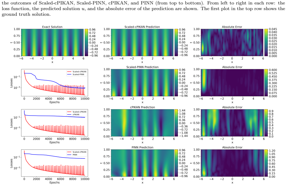
- Unscaled cPIKAN and PINN errors grow as the domain widens from $M=2$ to $M=6$, while Scaled-cPIKAN errors stay roughly constant, implying the method's accuracy is largely domain-independent.
- Scaled-cPIKAN estimates the unknown reaction coefficient in the inverse reaction-diffusion problem with about 99% lower relative error than the baselines even under noisy data, suggesting the scaling also improves parameter identification.
- Because Scaled-PINN outperforms PINN in several tests, the scaling is useful beyond KANs, although the Chebyshev version gains the most.
Reading between the lines
- An explicit affine map would let future work test whether the scaling's benefit is purely a conditioning effect: oscillatory solutions such as $\sin(a\pi x)$ on $[-M,M]$ become $\sin(a\pi M s)$ on $s\in[-1,1]$, so the method is effectively asking Chebyshev polynomials to resolve a higher-frequency function on their natural spectral grid.
- The same scaling idea presumably applies to other orthogonal-polynomial KAN bases that also have a native interval, and to temporal variables, which the paper keeps fixed at $[0,1]$; testing those extensions is a natural next step.
- The paper notes that very large domains beyond its tested range would need decomposition; combining per-subdomain affine maps with domain decomposition is an evident continuation that the current experiments do not yet cover.
Editorial analysis
A structured set of objections, weighed in public.
Referee Report
Summary. The paper proposes Scaled-cPIKAN, a Chebyshev-based physics-informed Kolmogorov-Arnold network that first rescales the spatial coordinates of a PDE to [-1,1]^d before training. The method is compared against cPIKAN, PINN, and a domain-scaled PINN on the diffusion, Helmholtz, Allen-Cahn, and forward/inverse reaction-diffusion equations, with relative L2 errors and training-loss histories reported for domain half-widths M = 2, 4, and 6. The authors conclude that Scaled-cPIKAN consistently outperforms the baselines, particularly on larger oscillatory domains and in noisy inverse problems.
Significance. If the reported improvements are reproducible, the contribution is a simple and practically relevant preprocessing step: an affine rescaling of the PDE before training a Chebyshev PIKAN. The paper deserves credit for matching parameter counts across methods in most comparisons and for evaluating accuracy against external analytic solutions, so the empirical comparisons are not circular. The breadth of evidence across four benchmark families is a strength. The main weaknesses are that the core coordinate transformation is never written down, all experiments are single runs without error bars, and one table contradicts the abstract's 'all test cases' claim; these issues currently prevent the reader from verifying the central mechanism.
major comments (4)
- [Section 3, Eqs. (12)-(18)] The central mechanism, the affine scaling of spatial variables, is never explicitly defined. The text introduces the scaled PDE in Eq. (12) with x̃ ∈ [-1,1]^d, but it does not give the map x → x̃, the chain-rule form of the scaled operators N^s and B^s, or the inverse map used to evaluate the network output on the original domain. Because the cKAN forward pass in Eq. (10) already applies tanh to its inputs, the only substantive difference between cPIKAN and Scaled-cPIKAN is precisely this coordinate transformation; if it is applied inconsistently to the residual, boundary, initial, or measurement terms, the comparisons in Tables 1-6 do not establish the claimed mechanism. This is especially acute in the inverse reaction-diffusion example of Section 4.4, where the scaling of the noisy data and source term is not specified and the reported κ errors differ from the baselines by three orders of magnitude; the reader cannot verify that this gap is caused by the scaling rather than by a different implicit treatment of the scaled data. Please write out the transformation and the scaled operator for at least one worked example, and specify how the network prediction is mapped back to the original coordinates before computing the error in Eq. (21).
- [Abstract; Table 5] The abstract claims that Scaled-cPIKAN 'significantly outperforms existing methods in all test cases,' but Table 5 (reaction-diffusion, forward, M = 2) reports a relative L2 error of 2.5 × 10^-2 for cPIKAN versus 2.7 × 10^-2 for Scaled-cPIKAN, i.e., the unscaled method is slightly better in that configuration. This contradiction should be resolved by either tempering the abstract and conclusion claims or explaining why this single M = 2 case is an exception. As written, the 'all test cases' statement is factually incorrect.
- [Tables 1-6] All tables report a single training run per configuration, with no standard deviations, seeds, or repeated trials. Given that the comparisons involve Adam optimization, randomly sampled collocation points, and loss landscapes that are sensitive to initialization, the reported differences—especially the three-order-of-magnitude gap in the inverse κ estimates of Table 6—cannot be distinguished from run-to-run variance. Please report statistics over multiple independent runs (at least 3-5 seeds) or clearly state that the tables are single-run exploratory results and adjust the strength of the conclusions accordingly.
- [Section 4.4, Eqs. (27)-(29)] In the inverse reaction-diffusion problem, Table 6 reports relative L2 errors for the source term f, but the text does not state how the predicted f is obtained from the network (e.g., by differentiating the approximate solution and evaluating N^s[ũ] = f̃) nor how the noisy scaled source term f^δ enters the loss. Please specify these details, because the scaling of f is part of the transformation that the paper claims is responsible for the improvement.
minor comments (7)
- [Section 4, Eq. (21)] The error metric is computed on the test set T* in the original domain; please state explicitly that the Scaled-cPIKAN output is first mapped back to the original coordinates before computing uP, and give the inverse mapping formula.
- [Table 2] The second block of Table 2 changes the header notation from (N_l, N_n, k) to (L, N, D); please unify the notation.
- [Table 4] PINN and Scaled-PINN report exactly the same relative L2 error (5.1 × 10^-1) for M = 2, 4, and 6; this suggests the models collapse to a trivial prediction, and the manuscript should comment on this behavior or verify the entries.
- [Section 4.4] The inverse problem uses only N_data = 10 measurement points; please specify how these points are selected and whether this is sufficient for the parameter estimation claims.
- [Figures 1-9 captions] The captions state that 'the first plot in the top row shows the ground truth solution,' which conflicts with the preceding description of the left column as the loss function; please correct the captions or the figure layout.
- [Section 4.1] The claim of 'several orders of magnitude higher accuracy' is stronger than the data for M = 2 (e.g., Table 1: Scaled-cPIKAN 4.3 × 10^-3 vs. cPIKAN 1.3 × 10^-2); please qualify the claim to be consistent with the reported orders of magnitude.
- [Section 3, Eq. (12)] The notation N^s and B^s is defined only verbally; at minimum, provide the definitions for one scalar example (e.g., the diffusion operator) to illustrate the chain rule.
Circularity Check
No circularity found: the claimed accuracy gains are measured against independent analytic solutions, and self-citations are not load-bearing.
full rationale
The paper's central claim is empirical: Scaled-cPIKAN is compared against analytic or manufactured ground-truth solutions for the diffusion, Helmholtz, Allen-Cahn, and reaction-diffusion problems. The relative L2 error in Eq. (21) is evaluated on a test set T* distinct from training points, against uE supplied by closed-form solutions such as u(x,t)=sin(pi x)exp(-pi^2 D t) and u(x,y)=sin(a1 pi x) sin(a2 pi y). No learned parameter is fit to these benchmark errors, and no reported 'prediction' is statistically forced by the training loss. The domain-scaling idea is described as a transformation in Eq. (12), but the paper never states the coordinate map or the chain-rule form of N^s; this omission makes the mechanism hard to reproduce, but it is not circular because the scaled operator is not defined in terms of the target solution or the reported error. Self-citations to the authors' earlier work (e.g., [33] in the survey of KAN implementations) are contextual and are not used to justify the scaling result. The abstract's 'all test cases' claim is internally weakened by Table 5, where cPIKAN reports 2.5e-2 and Scaled-cPIKAN reports 2.7e-2 at M=2, but this is an accuracy-claim inconsistency, not a derivation that consumes its own conclusion. Accordingly, no circular step can be exhibited with a specific reduction, and the appropriate finding is no significant circularity.
Assumptions & free parameters
free parameters (5)
- Residual loss weight lambda_res =
0.01, 0.5, or 1.0 per example
- Data, initial, and boundary loss weights =
1.0 or 0.0 depending on problem
- Collocation and data counts =
e.g., 2000/800, 4000/4000, 50000/400/200, 1200/10
- Network size (Nl, Nn, k) =
e.g., (2,8,5), (4,8,3), (4,20,5)
- Learning rate and training epochs =
1e-3 or 1e-4; 10,000 to 150,000 epochs
assumptions (4)
- standard math Kolmogorov-Arnold representation theorem: any continuous multivariate function can be written as sums and compositions of univariate functions.
- domain assumption Chebyshev polynomials are defined on [-1,1]; inputs must be normalized to that interval for stable training.
- domain assumption Manufactured benchmark solutions and their derived source terms are representative of real PDE challenges.
- domain assumption Adam optimization with fixed learning rate is sufficient to compare methods fairly.
Cite this review
Pith. "Pith review of Scaled-cPIKANs: Domain Scaling in Chebyshev-based Physics-informed Kolmogorov-Arnold Networks." pith.science (2026). https://pith.science/paper/S2ANE6OU
@misc{pith2026250102762,
  author       = {Pith},
  title        = {Pith review of: Scaled-cPIKANs: Domain Scaling in Chebyshev-based Physics-informed Kolmogorov-Arnold Networks},
  year         = {2026},
  howpublished = {\url{https://pith.science/paper/S2ANE6OU}},
  note         = {Machine review of arXiv:2501.02762}
}
abstract
Partial Differential Equations (PDEs) are integral to modeling many scientific and engineering problems. Physics-informed Neural Networks (PINNs) have emerged as promising tools for solving PDEs by embedding governing equations into the neural network loss function. However, when dealing with PDEs characterized by strong oscillatory dynamics over large computational domains, PINNs based on Multilayer Perceptrons (MLPs) often exhibit poor convergence and reduced accuracy. To address these challenges, this paper introduces Scaled-cPIKAN, a physics-informed architecture rooted in Kolmogorov-Arnold Networks (KANs). Scaled-cPIKAN integrates Chebyshev polynomial representations with a domain scaling approach that transforms spatial variables in PDEs into the standardized domain \([-1,1]^d\), as intrinsically required by Chebyshev polynomials. By combining the flexibility of Chebyshev-based KANs (cKANs) with the physics-driven principles of PINNs, and the spatial domain transformation, Scaled-cPIKAN enables efficient representation of oscillatory dynamics across extended spatial domains while improving computational performance. We demonstrate Scaled-cPIKAN efficacy using four benchmark problems: the diffusion equation, the Helmholtz equation, the Allen-Cahn equation, as well as both forward and inverse formulations of the reaction-diffusion equation (with and without noisy data). Our results show that Scaled-cPIKAN significantly outperforms existing methods in all test cases. In particular, it achieves several orders of magnitude higher accuracy and faster convergence rate, making it a highly efficient tool for approximating PDE solutions that feature oscillatory behavior over large spatial domains.
Figures


Figures from the paper (13 more)


Forward citations
Cited by 1 Pith paper
-
Augmented Physics-Based Li-ion Battery Model via Adaptive Ensemble Sparse Learning and Conformal Prediction
A hybrid battery model that learns sparse corrections to a reduced-order physics model reduces unseen-cycle voltage MSE by up to 46%, with conformal intervals above 90% coverage.
Reference graph
Works this paper leans on
-
[1]
Physics-informed neural networks: A deep learning framework for solving forward and inverse problems involving nonlinear partial differential equations
Maziar Raissi, Paris Perdikaris, and George E Karniadakis. Physics-informed neural networks: A deep learning framework for solving forward and inverse problems involving nonlinear partial differential equations. Journal of Computational physics , 378:686–707, 2019
2019
-
[2]
Physics-informed neural networks (pinns) for fluid mechanics: A review
Shengze Cai, Zhiping Mao, Zhicheng Wang, Minglang Yin, and George Em Karniadakis. Physics-informed neural networks (pinns) for fluid mechanics: A review. Acta Mechanica Sinica, 37(12):1727–1738, 2021
2021
-
[3]
Salah A Faroughi, Ramin Soltanmohammadi, Pingki Datta, Seyed Kourosh Mahjour, and Shirko Faroughi. Physics-informed neural networks with periodic activation functions for solute transport in heterogeneous porous media. Mathematics, 12(1): 63, 2023
work page 2023
-
[4]
Haoteng Hu, Lehua Qi, and Xujiang Chao. Physics-informed neural networks (pinn) for computational solid mechanics: Numerical frameworks and applications. Thin-Walled Structures, page 112495, 2024
work page 2024
-
[5]
Shahed Rezaei, Reza Najian Asl, Shirko Faroughi, Mahdi Asgharzadeh, Ali Harandi, Rasoul Najafi Koopas, Gottfried Laschet, Stefanie Reese, and Markus Apel. A finite operator learning technique for mapping the elastic properties of microstructures to their mechanical deformations. International Journal for Numerical Methods in Engineering , page e7637, 2024
work page 2024
-
[6]
Enhancing Arterial Blood Flow Simulations through Physics-Informed Neural Networks
Shivam Bhargava and Nagaiah Chamakuri. Enhancing arterial blood flow simulations through physics-informed neural networks. arXiv preprint arXiv:2404.16347 , 2024
work page Pith review arXiv 2024
-
[7]
Federica Caforio, Francesco Regazzoni, Stefano Pagani, Elias Karabelas, Christoph Augustin, Gundolf Haase, Gernot Plank, and Alfio Quarteroni. Physics-informed neural network estimation of material properties in soft tissue nonlinear biomechanical models. Computational Mechanics, pages 1–27, 2024
work page 2024
-
[8]
A physics-informed neural network to model the flow of dry particles
Pingki Datta, Nikhil Pawar, and Salah A Faroughi. A physics-informed neural network to model the flow of dry particles. In AGU Fall Meeting Abstracts , volume 2022, pages H52N–0633, 2022
work page 2022
Show all 45 references
-
[9]
From pinns to pikans: Recent advances in physics-informed machine learning
Juan Diego Toscano, Vivek Oommen, Alan John Varghese, Zongren Zou, Nazanin Ahmadi Daryakenari, Chenxi Wu, and George Em Karniadakis. From pinns to pikans: Recent advances in physics-informed machine learning. arXiv preprint arXiv:2410.13228, 2024
-
[10]
Physics-guided, physics-informed, and physics-encoded neural networks and operators in scientific com- puting: Fluid and solid mechanics
Salah A Faroughi, Nikhil M Pawar, Celio Fernandes, Maziar Raissi, Subasish Das, Nima K Kalantari, and Seyed Kourosh Mahjour. Physics-guided, physics-informed, and physics-encoded neural networks and operators in scientific com- puting: Fluid and solid mechanics. Journal of Com...
2024
-
[11]
Physics-informed machine learning for modeling multidimensional dynamics
Amirhassan Abbasi, Prashant N Kambali, Parham Shahidi, and C Nataraj. Physics-informed machine learning for modeling multidimensional dynamics. Nonlinear Dynamics, 112(24):21565–21585, 2024. 21
2024
-
[12]
Surrogate modeling of multi-dimensional premixed and non-premixed combustion using pseudo-time stepping physics-informed neural networks
Zhen Cao, Kai Liu, Kun Luo, Sifan Wang, Liang Jiang, and Jianren Fan. Surrogate modeling of multi-dimensional premixed and non-premixed combustion using pseudo-time stepping physics-informed neural networks. Physics of Fluids , 36(11), 2024
2024
-
[13]
Tackling the curse of dimensionality with physics-informed neural networks
Zheyuan Hu, Khemraj Shukla, George Em Karniadakis, and Kenji Kawaguchi. Tackling the curse of dimensionality with physics-informed neural networks. Neural Networks, 176:106369, 2024
2024
-
[14]
Understanding and mitigating gradient pathologies in physics-informed neural networks
Sifan Wang, Yujun Teng, and Paris Perdikaris. Understanding and mitigating gradient pathologies in physics-informed neural networks. arXiv preprint arXiv:2001.04536 , 2020
2001 arXiv
-
[15]
δ-pinns: physics-informed neural networks on complex geometries
Francisco Sahli Costabal, Simone Pezzuto, and Paris Perdikaris. δ-pinns: physics-informed neural networks on complex geometries. Engineering Applications of Artificial Intelligence , 127:107324, 2024
2024
-
[16]
Discontinuity computing using physics-informed neural networks
Li Liu, Shengping Liu, Hui Xie, Fansheng Xiong, Tengchao Yu, Mengjuan Xiao, Lufeng Liu, and Heng Yong. Discontinuity computing using physics-informed neural networks. Journal of Scientific Computing , 98(1):22, 2024
2024
-
[17]
Kan 2.0: Kolmogorov-arnold networks meet science
Ziming Liu, Pingchuan Ma, Yixuan Wang, Wojciech Matusik, and Max Tegmark. Kan 2.0: Kolmogorov-arnold networks meet science. arXiv preprint arXiv:2408.10205 , 2024
2024 arXiv
-
[18]
Kan: Kolmogorov-arnold networks
Ziming Liu, Yixuan Wang, Sachin Vaidya, Fabian Ruehle, James Halverson, Marin Soljaˇ ci´ c, Thomas Y Hou, and Max Tegmark. Kan: Kolmogorov-arnold networks. arXiv preprint arXiv:2404.19756 , 2024
2024 arXiv
-
[19]
A comprehensive and fair comparison between mlp and kan representations for differential equations and operator networks
Khemraj Shukla, Juan Diego Toscano, Zhicheng Wang, Zongren Zou, and George Em Karniadakis. A comprehensive and fair comparison between mlp and kan representations for differential equations and operator networks. arXiv preprint arXiv:2406.02917, 2024
2024 arXiv
-
[20]
On a constructive proof of kolmogorov’s superposition theorem
J¨ urgen Braun and Michael Griebel. On a constructive proof of kolmogorov’s superposition theorem. Constructive approxi- mation, 30:653–675, 2009
2009
-
[21]
On the representation of continuous functions of many variables by superposition of continuous functions of one variable and addition
Andrei Nikolaevich Kolmogorov. On the representation of continuous functions of many variables by superposition of continuous functions of one variable and addition. In Doklady Akademii Nauk, volume 114, pages 953–956. Russian Academy of Sciences, 1957
1957
-
[22]
Finite basis kolmogorov-arnold networks: domain decomposition for data-driven and physics-informed problems
Amanda A Howard, Bruno Jacob, Sarah H Murphy, Alexander Heinlein, and Panos Stinis. Finite basis kolmogorov-arnold networks: domain decomposition for data-driven and physics-informed problems. arXiv preprint arXiv:2406.19662 , 2024
2024
-
[23]
Relu-kan: New kolmogorov-arnold networks that only need matrix addition, dot multiplication, and relu
Qi Qiu, Tao Zhu, Helin Gong, Liming Chen, and Huansheng Ning. Relu-kan: New kolmogorov-arnold networks that only need matrix addition, dot multiplication, and relu. arXiv preprint arXiv:2406.02075 , 2024
2024 arXiv
-
[24]
Kkans: Kurkova-kolmogorov-arnold networks and their learning dynamics
Juan Diego Toscano, Li-Lian Wang, and George Em Karniadakis. Kkans: Kurkova-kolmogorov-arnold networks and their learning dynamics. arXiv preprint arXiv:2412.16738 , 2024
2024 arXiv
-
[25]
Kolmogorov-arnold networks are radial basis function networks
Ziyao Li. Kolmogorov-arnold networks are radial basis function networks. arXiv preprint arXiv:2405.06721 , 2024
2024 arXiv
-
[26]
Radial basis function neural network (rbfnn) approximation of cauchy inverse problems of the laplace equation
Farinaz Mostajeran and Seyed Mohammad Hosseini. Radial basis function neural network (rbfnn) approximation of cauchy inverse problems of the laplace equation. Computers & Mathematics with Applications , 141:129–144, 2023
2023
-
[27]
Wav-kan: Wavelet kolmogorov-arnold networks
Zavareh Bozorgasl and Hao Chen. Wav-kan: Wavelet kolmogorov-arnold networks. arXiv preprint arXiv:2405.12832 , 2024
2024 arXiv
-
[28]
A novel growing wavelet neural network algorithm for solving chemotaxis systems with blow-up
F Mostajeran and SM Hosseini. A novel growing wavelet neural network algorithm for solving chemotaxis systems with blow-up. Mathematical Methods in the Applied Sciences , 46(15):16255–16281, 2023
2023
-
[29]
Chebyshev polynomial-based kolmogorov-arnold networks: An efficient archi- tecture for nonlinear function approximation
Sidharth SS, Keerthana AR, Anas KP, et al. Chebyshev polynomial-based kolmogorov-arnold networks: An efficient archi- tecture for nonlinear function approximation. arXiv preprint arXiv:2405.07200 , 2024
2024 arXiv
-
[30]
Control of a hydraulic generator regulating system using chebyshev-neural-network-based non-singular fast terminal sliding mode method
Fawaz E Alsaadi, Amirreza Yasami, Hajid Alsubaie, Ahmed Alotaibi, and Hadi Jahanshahi. Control of a hydraulic generator regulating system using chebyshev-neural-network-based non-singular fast terminal sliding mode method. Mathematics, 11 (1):168, 2022
2022
-
[31]
Development of a novel activation function based on chebyshev polynomials: an aid for classification and denoising of images
M Deepthi, GNVR Vikram, and P Venkatappareddy. Development of a novel activation function based on chebyshev polynomials: an aid for classification and denoising of images. The Journal of Supercomputing , 79(18):20515–20531, 2023
2023
-
[32]
Physics-informed kolmogorov-arnold network with chebyshev polynomials for fluid mechanics
Chunyu Guo, Lucheng Sun, Shilong Li, Zelong Yuan, and Chao Wang. Physics-informed kolmogorov-arnold network with chebyshev polynomials for fluid mechanics. arXiv preprint arXiv:2411.04516 , 2024
2024 arXiv
-
[33]
Epi-ckans: Elasto-plasticity informed kolmogorov-arnold networks using chebyshev polynomials
Farinaz Mostajeran and Salah A Faroughi. Epi-ckans: Elasto-plasticity informed kolmogorov-arnold networks using chebyshev polynomials. arXiv preprint arXiv:2410.10897 , 2024
2024 arXiv
-
[34]
Kolmogorov arnold informed neural network: A physics-informed deep learning framework for solving pdes based on kolmogorov arnold networks
Yizheng Wang, Jia Sun, Jinshuai Bai, Cosmin Anitescu, Mohammad Sadegh Eshaghi, Xiaoying Zhuang, Timon Rabczuk, and Yinghua Liu. Kolmogorov arnold informed neural network: A physics-informed deep learning framework for solving pdes based on kolmogorov arnold networks. arXiv pre...
2024 arXiv
-
[35]
Spikans: Separable physics-informed kolmogorov-arnold networks
Bruno Jacob, Amanda A Howard, and Panos Stinis. Spikans: Separable physics-informed kolmogorov-arnold networks. arXiv preprint arXiv:2411.06286, 2024
2024 arXiv
-
[36]
Partial differential equations , volume 19
Lawrence C Evans. Partial differential equations , volume 19. American Mathematical Society, 2022
2022
-
[37]
Sur les probl` emes aux d´ eriv´ ees partielles et leur signification physique.Princeton university bulletin , pages 49–52, 1902
Jacques Hadamard. Sur les probl` emes aux d´ eriv´ ees partielles et leur signification physique.Princeton university bulletin , pages 49–52, 1902
1902
-
[38]
Solutions of ill-posed problems
Andrey Nikolayevich Tikhonov. Solutions of ill-posed problems. VH Winston and Sons , 1977
1977
-
[39]
Deep learning, volume 1
Yoshua Bengio, Ian Goodfellow, and Aaron Courville. Deep learning, volume 1. MIT press Cambridge, MA, USA, 2017
2017
-
[40]
Pattern recognition and machine learning , volume 4
Christopher M Bishop and Nasser M Nasrabadi. Pattern recognition and machine learning , volume 4. Springer, 2006
2006
-
[41]
A brief review of feed-forward neural networks
Murat H Sazlı. A brief review of feed-forward neural networks. Communications Faculty of Sciences University of Ankara Series A2-A3 Physical Sciences and Engineering , 50(01), 2006
2006
-
[42]
Introduction to multi-layer feed-forward neural networks
Daniel Svozil, Vladimir Kvasnicka, and Jiri Pospichal. Introduction to multi-layer feed-forward neural networks. Chemomet- rics and intelligent laboratory systems , 39(1):43–62, 1997
1997
-
[43]
Approximation by superpositions of a sigmoidal function
George Cybenko. Approximation by superpositions of a sigmoidal function. Mathematics of control, signals and systems , 2 (4):303–314, 1989
1989
-
[44]
Chebyshev polynomials
Theodore J Rivlin. Chebyshev polynomials. Courier Dover Publications, 2020
2020
-
[45]
The kolmogorov–arnold representation theorem revisited
Johannes Schmidt-Hieber. The kolmogorov–arnold representation theorem revisited. Neural networks, 137:119–126, 2021. 22 Appendix A. Additional Supporting Figures Figure A.1: Comparison of the solutions predicted for the Allen-Cahn equation (Example 4.3) in a supervised version...
2021
Reviewed August 10, 2026 · model on record in the stance chip above.
Discussion (0). Continue with ORCID to comment.