REVIEW 5 major objections 6 minor 1 cited by
Separable Geodesic Lagrangian Monte Carlo for Inference in 2-Way Covariance Models
T0 review · 5 major / 6 minor · reviewed 2026-08-10 · deepseek-v4-flash
Pith's one-line read A geodesic Hamiltonian sampler puts separable-covariance MCMC on par with Gibbs
desk verdict Regularized SGLMC is a plausible new MCMC tool for separable covariances, but the orthogonal/weighted variants sample a conditional slice rather than the posterior, and the printed algorithm has enough errors that the paper needs major revision before it can be trusted. read the letter →
The pith
A machine-rendered reading of the paper's core claim, the machinery that carries it, and where it could break.
The reading
What carries the argument
The load-bearing object is the affine-invariant metric on positive-definite matrices, $g_\Sigma(S_1,S_2)=\operatorname{tr}(\Sigma^{-1}S_1\Sigma^{-1}S_2)$, together with its closed-form geodesic exponential map $\exp_\Sigma(tV)=\Sigma^{1/2}\exp(t\Sigma^{-1/2}V\Sigma^{-1/2})\Sigma^{1/2}$. The paper pulls this metric back through the Kronecker map, identifies the resulting degeneracy by a rank-one determinant calculation, and repairs it with four metrics: regularized $G^\otimes_\alpha$, orthogonal $G^O$, weighted $G^W$, and product $G^\times$. The other essential mechanism is the Pitsianis–Van Loan decomposition, which rewrites the sample sum of squares as a sum of Kronecker products so that log-likelihood, gradients, and Gibbs full conditionals factor into component traces; this is what makes both the geodesic gradients and the comparison Gibbs sampler computationally tractable.
What would settle it
Run SGLMC-O on a small dataset with known true $\Sigma_1,\Sigma_2$, then compare the normalized posterior of $\Sigma_2$ against a very long Gibbs run with the same inverse-Wishart prior; if the Metropolis acceptance rate depends on trajectory direction, or if the normalized SGLMC marginals drift from the Gibbs marginals, the constrained leapfrog is not reversible for the claimed target.
Extended reading notes
Core claim
On the product manifold $P(d_1)\times P(d_2)$, the pullback of the affine-invariant metric under the map $(\Sigma_1,\Sigma_2)\mapsto \Sigma_1\otimes\Sigma_2$ is degenerate, because $\lvert c\Sigma_1\rvert \lvert c^{-1}\Sigma_2\rvert = \lvert\Sigma_1\rvert\lvert\Sigma_2\rvert$ creates a scale direction of zero norm. The paper resolves this degeneracy in four ways, regularizing the off-diagonal block, orthogonalizing with the projection $P_{\Sigma_2}$, weighting the blocks, or simply taking the product metric, and then asserts Proposition 2.3: under every one of these metrics, the geodesic is $\Sigma(t)=\Sigma_1(t)\otimes\Sigma_2(t)$ with $\Sigma_i(t)=\exp_{\Sigma_i(0)}(t V_i(0))$ the affine-invariant exponential map. This lets a geodesic Hamiltonian Monte Carlo sampler split into two lower-dimensional factor updates, with velocities drawn from matrix-normal-type distributions and Riemannian gradients computed through the Pitsianis–Van Loan decomposition. The paper's experiments compare the resulting SGLMC sampler with Gibbs and with a general-purpose HMC implementation and conclude that the constrained (orthogonal) and weighted metrics give higher effective sample size per iteration than the product metric while tracking Gibbs posterior summaries.
Load-bearing premise
The sampler's correctness rests on the assumption, inherited from earlier Lagrangian Monte Carlo work without a proof for this specific case, that the generalized leapfrog integrator with a position-dependent metric is reversible and samples the intended posterior even when the block-diagonal orthogonal metric is combined with the projection constraint on $\Sigma_2$; the printed Algorithm 2 also contains typos in the projection and final half-kick that an implementation must repair.
Editorial extensions
If this is right
- Because the geodesic on the full Kronecker covariance is the Kronecker product of two independent affine-invariant geodesics, each leapfrog step costs two smaller matrix exponentials, $O(d_1^3+d_2^3)$, instead of one exponential on $d_1d_2$-dimensional matrices.
- For the orthogonal, weighted, and product metrics, the velocity and gradient updates can be written in matrix form without forming the full metric tensor, avoiding a naive $O((d_1^2+d_2^2)^3)$ inversion cost.
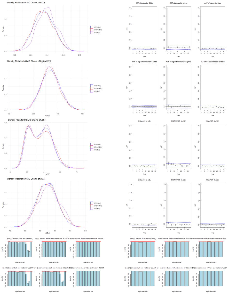
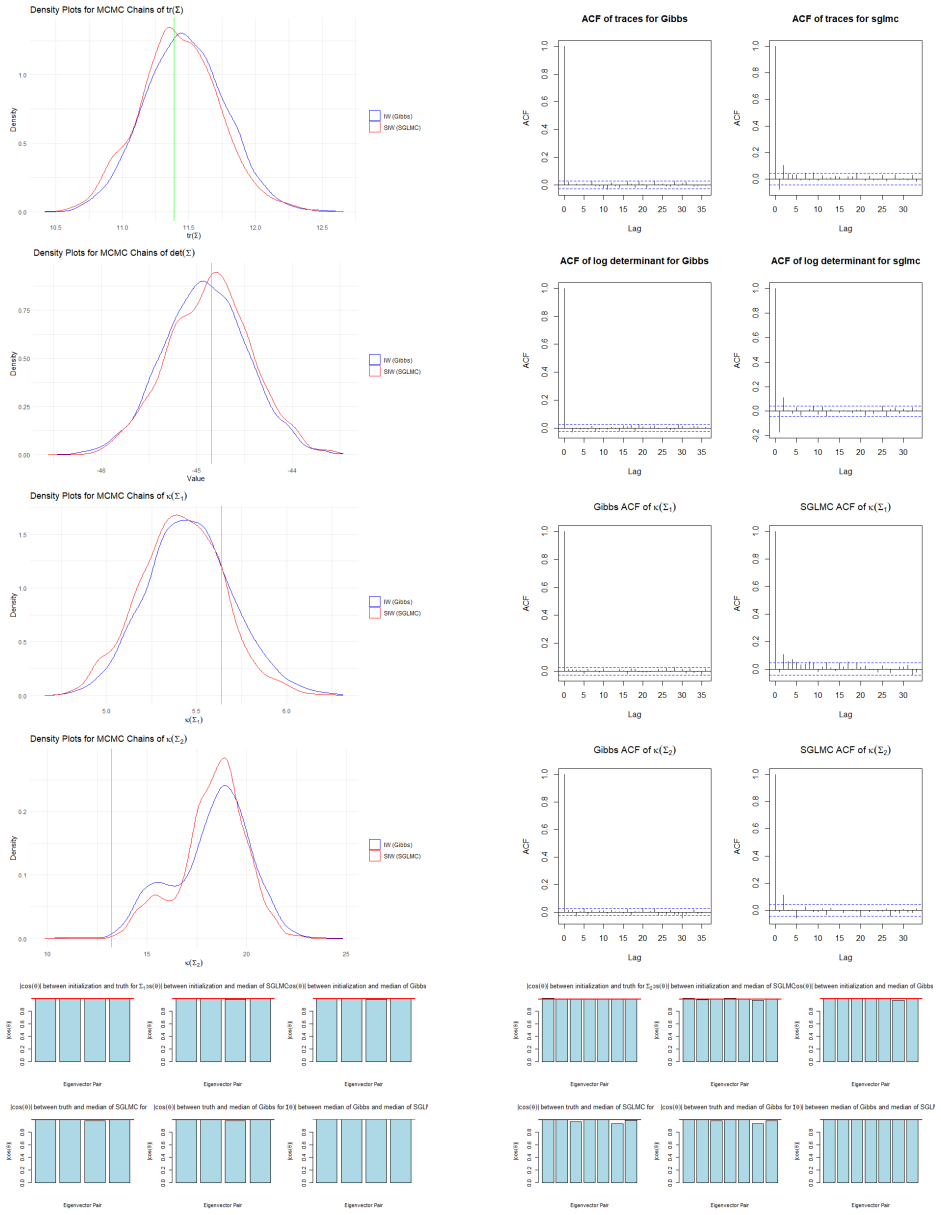
- With inverse-Wishart priors, SGLMC posterior densities for trace, log-determinant, and condition number agree with Gibbs; the $\lvert\Sigma_2\rvert=1$ constraint affects only the scale indeterminacy and disappears after normalizing Gibbs samples.
- The experiments indicate that the regularized metric with $\alpha=0.95$ and the orthogonal or weighted metrics produce higher effective sample sizes per iteration than the product metric, and that sampler autocorrelation improves as $\alpha$ grows toward 1.
- The Pitsianis–Van Loan decomposition yields full conditional distributions for the components, giving a direct conjugate Gibbs comparator and gradients with cost $O(r\,d_{\max}^3)$ rather than $O(n\,d_{\max}^3)$ for the matrix-normal likelihood.
Reading between the lines
- If Proposition 2.3 extends to higher-order Kronecker products, the same component-wise exponential-map construction gives an immediate tensor generalization; the paper notes only that the P-VL gradient cost would then grow, so the practical bottleneck would move from geometry to gradient computation.
- The near-independence of posterior marginals across $\alpha$ values suggests the metric is acting primarily as a sampler-tuning device rather than as part of the statistical model, so one could treat metric choice and target distribution as separate design decisions.
- As printed, Algorithm 2 applies the projection $P_{\Sigma_1}$ in the $\Sigma_2$ velocity update and reuses $q_j$ rather than $q_{j+1}$ in the final half-kick; these typos must be corrected before the empirical claims can be reproduced, and the paper does not flag them.
- A fully adaptive version could replace the static leapfrog length $L$ with the log-map termination criterion sketched in the supplement; testing whether that recovers no-U-turn-style efficiency on the constrained metric would be a natural follow-up.
Signed reviews
Editorial analysis
A structured set of objections, weighed in public.
Referee Report
Summary. The paper develops Separable Geodesic Lagrangian Monte Carlo (SGLMC) for Bayesian inference in matrix-normal models with separable covariance Sigma = Sigma1 ⊗ Sigma2. The authors construct four metrics on P(d1) × P(d2): a regularized pullback of the affine-invariant metric, an orthogonalized block-diagonal metric GO, a weighted variant GW, and the product metric G×. Proposition 2.3 claims that under all of these metrics the geodesic flow factors into independent affine-invariant geodesics on P(d1) and P(d2). Using the Pitsianis–Van Loan decomposition, the paper gives Gibbs full conditionals and likelihood gradients, presents Algorithms 1 and 2, and reports numerical comparisons with Gibbs and Stan, including an application to the Wisconsin breast-cancer data.
Significance. Proposition 2.3 is potentially a significant simplification: if valid, geodesic HMC on the Kronecker-structured parameter space can be implemented by independent SPD geodesics, and the P-VL-based gradient computations avoid dense Kronecker algebra. The paper also provides a useful full-conditional decomposition and extensive empirical documentation. However, the manuscript as written does not establish that the orthogonal or weighted samplers target the claimed posterior, and the printed algorithms contain internal inconsistencies. These issues are load-bearing for the validity and efficiency claims, although the core geometric idea appears salvageable.
major comments (5)
- [Sec. 4.2, Fig. 5, Table 1] The claim that the |Σ2|=1 constraint of GO and GW introduces only a bias 'equivalent to normalizing samples of Σ2 with the Gibbs sampler' is not correct for the IW priors in (22). In the identified parametrization (A,U) = (|Σ2|^{1/d2}Σ1, Σ2/|Σ2|^{1/d2}), the marginal posterior of (A,U) is obtained by integrating over the scale s; for the priors (22) the s-dependence of the posterior is exp[-γ/(2d1 s)tr(A^{-1}) - γs/(2d2)tr(U^{-1}) - (s/2)tr(A^{-1}Σ_k A_k tr(U^{-1}B_k))] times s^{d1(d1+1)/2 - d2(d2+1)/2 + 1}, which does not factor as h(s)g(A,U). Hence the slice |Σ2|=1, which is the stationary distribution of the constrained sampler, is not proportional to the normalized-Gibbs target, and the high ESS/it values for GO and GW in Table 1 and the agreement in Figure 5 are not evidence that these variants sample the posterior. A concrete minimal check is d1=d2=1, where normalized Gibbs targets the posterior of the product σ1σ2 while the slice target is the conditional of σ1 given σ2=1.
- [Sec. 4.2, Algorithm 2] The printed generalized leapfrog is internally inconsistent. In the second half-kick, the Σ2 velocity is updated with PΣ1 instead of PΣ2, the gradients are evaluated at qj instead of qj+1, and the velocity used is V^{(j)} instead of V^{(j+1/2)}; the two half-kick lines for V2 are identical. Such an update is neither reversible nor symplectic as written, and no detailed-balance proof is supplied for the projected, position-dependent metric. The manuscript therefore does not substantiate the claim that SGLMC-O samples any stated target distribution, and the algorithm cannot be run as printed.
- [Prop. 3.2, Eqs. (25)-(26)] The displayed gradients are not gradients of the negative log-likelihood. For the log-likelihood ℓ, one has ∂ℓ/∂Σ1 = -(d2+n)/2 Σ1^{-1} + (1/2)Σ_k tr(Σ2^{-1}B_k) Σ1^{-1}A_kΣ1^{-1}; the negative log-likelihood gradient is the negative of this expression. Equations (25)-(26) print the log-likelihood gradient instead. Since the leapfrog updates in Algorithm 2 require the gradient of πH = -log π - (1/2)log|G|, a sign error here changes the dynamics from descending to ascending the potential and, if implemented as printed, invalidates the sampler's stationary distribution.
- [Lemma 2.2, Eq. (11)] The proposed orthogonal map, PΣ2(V2) = V2 - tr(V2Σ2^{-1})/d2 V2, is not a projection and does not remove the cross term in Proposition 2.1; it merely rescales V2. The vectorized form P = I - vec(Σ2)vec(Σ2)^T/d2 projects along the Euclidean inner product with vec(Σ2) rather than along Σ2 under the affine-invariant metric. The correct projection enforcing tr(Σ2^{-1}V2)=0 is V2 - tr(Σ2^{-1}V2)/d2 Σ2. In addition, the coefficients in GO in Eq. (11) and in Lemma 2.2 are swapped relative to Proposition 2.1 and relative to the velocity scales and Riemannian gradients used in Algorithm 2. These inconsistencies affect both the geometric derivation and the actual implementation of the main orthogonal sampler.
- [Lemma 2.3, Eq. (31)] The determinant statement for GO and GW is ambiguous. For the full block-diagonal metric (11), the determinant is proportional to |Σ1|^{-(d1+1)}|Σ2|^{-(d2+1)}, not solely |Σ1|^{-(d1+1)}; the statement in Lemma 2.3 can only hold on the submanifold |Σ2|=1, for which no determinant computation is provided. Because the Hamiltonian (31) contains -(1/2)log|G(q)|, the invariant measure of the constrained sampler depends on which determinant is used. As written, whether SGLMC-O targets π(q) restricted to the slice, the marginal of the identified parameters, or some other measure is not well defined.
minor comments (6)
- [Prop. 2.2] The bottom-left block of G⊗ appears to be vec(Σ2^{-1})vec(Σ2^{-1})^T, which is not the transpose of the top-right block; it should be vec(Σ2^{-1})vec(Σ1^{-1})^T.
- [Sec. 8, proof of Prop. 2.3] The symbols P1 and P2 are used in place of Σ1 and Σ2 in several equations in the Euler-Lagrange proof, making the argument harder to follow.
- [Algorithm 1] The velocity update uses G(q(1)) throughout and refers to q(j+1/2), which is never defined; this should be corrected to match a standard generalized leapfrog.
- [Algorithm 2] The notation d^{1/2}_{-k} in the velocity sampling step is undefined; it should be d_{3-k}^{-1/2} or an equivalent explicit expression.
- [Secs. 5 and 8.5] The paper states that the propriety of the reference prior 'was not investigated in this paper and remains questionable' but still uses the reference prior in the real-data example; this example should be labeled as exploratory unless propriety is established.
- [Table 1] Table 1 reports ESS/it for log|Σ2| and log|Σ| for GO and GW even though |Σ2|=1 makes these statistics constant under the constraint; reporting these values is not informative and should be removed or replaced with identifiable statistics.
Circularity Check
No significant circularity: the SGLMC derivation relies on standard external affine-invariant geometry and is benchmarked against Gibbs/Stan; no fitted parameter is renamed as a prediction.
full rationale
The paper's central derivation chain is self-contained relative to established, externally sourced geometry. The Kronecker pullback metric, its degeneracy (Proposition 2.2), and the regularized/orthogonal/weighted/product variants (Lemma 2.1, Lemma 2.2) are derived from the paper's own equations using the affine-invariant metric of Moakher-Zerai and the Pitsianis-Van Loan decomposition. Proposition 2.3 is proven by checking that product-manifold geodesics satisfy the Euler-Lagrange equations of the coupled regularized metric; together with uniqueness of the geodesic ODE this is a valid sufficiency argument, not a circular definition. The sampler's stationary distribution correctly targets pi(q): in Eq. (31), the (1/2) log|G(q)| term cancels the sqrt(|G(q)|) normalization of the velocity distribution, so the position marginal is the full posterior on the constrained or unconstrained slice as stated. No fitted parameter is used to produce the geodesic equations; alpha and omega are tuning/design parameters, and the empirical ESS/it comparisons in Table 1 and posterior comparisons against Gibbs and Stan are independent external benchmarks, not predictions constructed from the same fitted values. The paper transparently acknowledges the |Sigma2|=1 constraint bias and compares to normalized Gibbs samples; whether that equivalence is mathematically exact is a correctness question, not circularity. Self-citation is not load-bearing: [16] and [21] are external prior works by other authors. Two non-circular concerns are noted per the review rule: the reference prior propriety is explicitly left uninvestigated (Section 5, Section 8.5), and Algorithm 2 contains an apparent typo (P_Sigma1 applied to the V2 update and qj reused in the final half-kick), which is a reproducibility risk rather than a circular step.
Assumptions & free parameters
free parameters (4)
- regularization parameter alpha =
0.95 (recommended); 0 <= alpha < 1
- leapfrog steps L =
10 in all experiments
- dual averaging target a0 =
0.8, 0.85, 0.6, 0.7 across experiments
- weight omega in GW =
not evaluated
assumptions (6)
- domain assumption The affine-invariant metric g_Sigma(S1,S2)=tr(Sigma^-1 S1 Sigma^-1 S2) defines the geometry of SPD matrices
- standard math The exponential map for the affine-invariant metric is Sigma(t)=Sigma^(1/2) exp(t Sigma^(-1/2) V Sigma^(-1/2)) Sigma^(1/2)
- ad hoc to paper The regularized and orthogonalized pullback metrics produce the same geodesics as the product manifold and have the stated determinant formulas
- domain assumption The generalized leapfrog integrator for Lagrangian Monte Carlo yields a reversible sampler with stationary distribution proportional to exp(-piH(q)) sqrt(|G(q)|)
- standard math The Pitsianis-Van Loan decomposition exactly represents sum_i y_i y_i^T as sum_k A_k tensor B_k
- ad hoc to paper The reference prior is proper for the models used
Cite this review
Pith. "Pith review of Separable Geodesic Lagrangian Monte Carlo for Inference in 2-Way Covariance Models." pith.science (2026). https://pith.science/paper/K2TA3JJZ
@misc{pith2026250104913,
  author       = {Pith},
  title        = {Pith review of: Separable Geodesic Lagrangian Monte Carlo for Inference in 2-Way Covariance Models},
  year         = {2026},
  howpublished = {\url{https://pith.science/paper/K2TA3JJZ}},
  note         = {Machine review of arXiv:2501.04913}
}
read the original abstract
Matrix normal models have an associated 4-tensor for their covariance representation. The covariance array associated with a matrix normal model is naturally represented as a Kronecker-product structured covariance associated with the vector normal, also known as separable covariance matrices. Separable covariance matrices have been studied extensively in the context of multiway data, but little work has been done within the scope of MCMC beyond Gibbs sampling. This paper aims to fill this gap by considering the pullback geometry induced from the Kronecker structure of the parameter space to develop a geodesic Hamiltonian Monte Carlo sampler.
Figures


Figures from the paper (19 more)





Forward citations
Cited by 1 Pith paper
-
Testing Covariance Separability in High Dimensions
Separability of high-dimensional matrix covariances can be tested by Monte Carlo sphericity after separable MLE whitening, with an angular version robust to heavy-tailed elliptical laws and consistency under dense alt...
Reference graph
Works this paper leans on
-
[1]
James O Berger, Dongchu Sun, and Chengyuan Song. Bayesian analysis of the covariance matrix of a multivariate normal distribution with a new class of priors. Annals of Statistics , 48(4):2381–2403, 2020. 16
work page 2020
-
[2]
Generalizing the no-u-turn sampler to Riemannian manifolds
Michael J Betancourt. Generalizing the no-u-turn sampler to Riemannian manifolds. arXiv preprint arXiv:1304.1920, 2013. 17, 23
arXiv 1920
-
[3]
Florent Bouchard, Arnaud Breloy, Ammar Mian, and Guillaume Ginolhac. On-line Kronecker product structured covariance estimation with Riemannian geometry for t-distributed data. In 2021 29th European Signal Processing Conference (EUSIPCO), pages 856–859. IEEE, 2021. 9
work page 2021
-
[4]
Geodesic Monte Carlo on embedded manifolds
Simon Byrne and Mark Girolami. Geodesic Monte Carlo on embedded manifolds. Scandinavian Journal of Statistics , 40(4):825–845, 2013. 2, 5, 10
work page 2013
-
[5]
Stan: A probabilistic programming language
Bob Carpenter, Andrew Gelman, Matthew D Hoffman, Daniel Lee, Ben Goodrich, Michael Be- tancourt, Marcus A Brubaker, Jiqiang Guo, Peter Li, and Allen Riddell. Stan: A probabilistic programming language. Journal of Statistical Software , 76, 2017. 3, 23
work page 2017
-
[6]
The mle algorithm for the matrix normal distribution
Pierre Dutilleul. The mle algorithm for the matrix normal distribution. Journal of Statistical Computation and Simulation , 64(2):105–123, 1999. 23
work page 1999
-
[7]
Estimation and testing for separable variance–covariance structures
Pierre Dutilleul. Estimation and testing for separable variance–covariance structures. Wiley Interdisciplinary Reviews: Computational Statistics , 10(4):e1432, 2018. 2
work page 2018
-
[8]
Herbert Federer. Geometric Measure Theory. Springer, 2014. 6
work page 2014
Show all 43 references
-
[9]
Separable factor analysis with applications to mortality data
Bailey K Fosdick and Peter D Hoff. Separable factor analysis with applications to mortality data. Annals of Applied Statistics , 8(1):120, 2014. 2
2014
-
[10]
Separable approximations of space-time covariance matrices
Marc G Genton. Separable approximations of space-time covariance matrices. Environmetrics: The Official Journal of the International Environmetrics Society , 18(7):681–695, 2007. 2
2007
-
[11]
Riemann manifold langevin and Hamiltonian Monte Carlo methods
Mark Girolami and Ben Calderhead. Riemann manifold langevin and Hamiltonian Monte Carlo methods. Journal of the Royal Statistical Society Series B: Statistical Methodology , 73(2):123–214, 2011. 2 27
2011
-
[12]
Robust Kronecker product pca for spatio-temporal covariance estimation
Kristjan Greenewald and Alfred O Hero. Robust Kronecker product pca for spatio-temporal covariance estimation. IEEE Transactions on Signal Processing , 63(23):6368–6378, 2015. 3
2015
-
[13]
Matrix variate distributions
Arjun K Gupta and Daya K Nagar. Matrix variate distributions . Chapman and Hall/CRC,
-
[14]
On Riemannian optimization over positive definite matrices with the Bures-Wasserstein geometry
Andi Han, Bamdev Mishra, Pratik Kumar Jawanpuria, and Junbin Gao. On Riemannian optimization over positive definite matrices with the Bures-Wasserstein geometry. Advances in Neural Information Processing Systems , 34:8940–8953, 2021. 26
2021
-
[15]
Separable covariance arrays via the tucker product, with applications to multi- variate relational data
Peter D Hoff. Separable covariance arrays via the tucker product, with applications to multi- variate relational data. Bayesian Analysis, 6(2):179 – 196, 2011. 2
2011
-
[16]
Geodesic Lagrangian Monte Carlo over the space of positive definite matrices: with application to Bayesian spectral density estimation
Andrew Holbrook, Shiwei Lan, Alexander Vandenberg-Rodes, and Babak Shahbaba. Geodesic Lagrangian Monte Carlo over the space of positive definite matrices: with application to Bayesian spectral density estimation. Journal of Statistical Computation and Simulation , 88(5):982–10...
2018
-
[17]
Hoff, and David B
Michael Jauch, Peter D. Hoff, and David B. Dunson. Random orthogonal matrices and the cayley transform. Bernoulli, 26(2):1560 – 1586, 2020. 2
2020
-
[18]
Hoff, and David B
Michael Jauch, Peter D. Hoff, and David B. Dunson. Monte Carlo simulation on the stiefel manifold via polar expansion. Journal of Computational and Graphical Statistics , 30(3):622– 631, 2021. 2
2021
-
[19]
Springer, 2008
J¨ urgen Jost and Jeurgen Jost.Riemannian Geometry and Geometric Analysis , volume 42005. Springer, 2008. 43
2008
-
[20]
Kronecker product and svd approximations in image restora- tion
Julie Kamm and James G Nagy. Kronecker product and svd approximations in image restora- tion. Linear Algebra and its Applications , 284(1-3):177–192, 1998. 3
1998
-
[21]
Markov chain Monte Carlo from lagrangian dynamics
Shiwei Lan, Vasileios Stathopoulos, Babak Shahbaba, and Mark Girolami. Markov chain Monte Carlo from lagrangian dynamics. Journal of Computational and Graphical Statistics , 24(2):357–378, 2015. 2, 17 28
2015
-
[22]
Spherical Hamiltonian Monte Carlo for con- strained target distributions
Shiwei Lan, Bo Zhou, and Babak Shahbaba. Spherical Hamiltonian Monte Carlo for con- strained target distributions. In International Conference on Machine Learning , pages 629–
-
[23]
Smooth manifolds
John M Lee and John M Lee. Smooth manifolds. Springer, 2012. 38
2012
-
[24]
A Bayesian factor model for spatial panel data with a separable covariance approach
Samantha Leorato and Maura Mezzetti. A Bayesian factor model for spatial panel data with a separable covariance approach. Bayesian Analysis, 16(2):489–519, 2021. 2
2021
-
[25]
Riemannian geometry of symmetric positive definite matrices via cholesky de- composition
Zhenhua Lin. Riemannian geometry of symmetric positive definite matrices via cholesky de- composition. SIAM Journal on Matrix Analysis and Applications , 40(4):1353–1370, 2019. 26
2019
-
[26]
The commutation matrix: some properties and applica- tions
Jan R Magnus and Heinz Neudecker. The commutation matrix: some properties and applica- tions. The Annals of Statistics , 7(2):381–394, 1979. 40
1979
-
[27]
Matrix differential calculus with applications to simple, hadamard, and Kronecker products
Jan R Magnus and Heinz Neudecker. Matrix differential calculus with applications to simple, hadamard, and Kronecker products. Journal of Mathematical Psychology, 29(4):474–492, 1985. 40
1985
-
[28]
Matrix Differential Calculus with Applications in Statis- tics and Econometrics
Jan R Magnus and Heinz Neudecker. Matrix Differential Calculus with Applications in Statis- tics and Econometrics . John Wiley & Sons, 2019. 16
2019
-
[29]
Information geometry and asymptotics for Kronecker covariances
Andrew McCormack and Peter Hoff. Information geometry and asymptotics for Kronecker covariances. arXiv preprint arXiv:2308.02260 , 2023. 2, 9
2023 arXiv
-
[30]
Carl D. Meyer. Matrix Analysis and Applied Linear Algebra . SIAM, 2023. 42
2023
-
[31]
The Riemannian geometry of the space of positive-definite matrices and its application to the regularization of positive-definite matrix-valued data
Maher Moakher and Mourad Z´ era ¨ ı. The Riemannian geometry of the space of positive-definite matrices and its application to the regularization of positive-definite matrix-valued data. Jour- nal of Mathematical Imaging and Vision , 40(2):171–187, 2011. 7, 18, 20, 44, 46
2011
-
[32]
The imbedding problem for Riemannian manifolds
John Nash. The imbedding problem for Riemannian manifolds. Annals of mathematics , 63(1):20–63, 1956. 5
1956
-
[33]
Mcmc using Hamiltonian dynamics
Radford M Neal et al. Mcmc using Hamiltonian dynamics. Handbook of Markiv Chain Monte Carlo, 2(11):2, 2011. 2, 17 29
2011
-
[34]
Rotation invariant householder parameterization for Bayesian pca
Rajbir Nirwan and Nils Berchtold. Rotation invariant householder parameterization for Bayesian pca. In Kamalika Chaudhuri and Ruslan Salakhutdinov, editors, Proceedings of the 36th International Conference on Machine Learning (Proceedings of Machine Learning Research, Vol. 97)...
2019
-
[35]
Rotation invariant householder parameterization for Bayesian PCA
Rajbir Nirwan and Nils Bertschinger. Rotation invariant householder parameterization for Bayesian PCA. In Kamalika Chaudhuri and Ruslan Salakhutdinov, editors, Proceedings of the 36th International Conference on Machine Learning , volume 97 of Proceedings of Machine Learning R...
2019
-
[36]
N. P. Pitsanis. The Kronecker product in approximation and fast transform generation . PhD thesis, Cornell University, Ithaca, NY, 1997. 13
1997
-
[37]
General Bayesian inference over the stiefel manifold via the givens transform.Bayesian Analysis, 16(2),
Arya Pourzanjani, Richard M Jiang, Brian Mitchell, Paul J Atzberger, and L Petzold. General Bayesian inference over the stiefel manifold via the givens transform.Bayesian Analysis, 16(2),
-
[38]
A Matrix Handbook for Statisticians
George AF Seber. A Matrix Handbook for Statisticians . John Wiley & Sons, 2008. 19
2008
-
[39]
C. F. Van Loan and N. Pitsianis. Approximation with Kronecker products. In Marc S. Moonen, Gene H. Golub, and Bart L. R. De Moor, editors,Linear Algebra for Large Scale and Real-Time Applications, pages 293–314. Springer Netherlands, 1993. 13
1993
-
[40]
Geodesic convexity and covariance estimation
Ami Wiesel. Geodesic convexity and covariance estimation. IEEE Transactions on Signal Processing, 60(12):6182–6189, 2012. 2
2012
-
[41]
William Wolberg, Olvi Mangasarian, Nick Street, and W. Street. Breast Cancer Wisconsin (Di- agnostic). UCI Machine Learning Repository, 1995. DOI: https://doi.org/10.24432/C5DW2B. 3, 25
1995 doi
-
[42]
Estimation of a covariance matrix using the reference prior
Ruoyong Yang and James O Berger. Estimation of a covariance matrix using the reference prior. The Annals of Statistics , pages 1195–1211, 1994. 15
1994
-
[43]
The Schur Complement and Its Applications , volume 4
Fuzhen Zhang. The Schur Complement and Its Applications , volume 4. Springer Science & Business Media, 2006. 11, 42 30 Figure 2: Density and corresponding ACFs plots of the traces, determinants for samples of Σ, and the condition numbers for samples of Σ 1, Σ2 from SGLMC, Gibb...
2006
Reviewed August 10, 2026 · model on record in the stance chip above.
Discussion (0). Continue with ORCID to comment.