REVIEW 4 major objections 7 minor 64 references
Progressive Supervision via Label Decomposition: An Long-Term and Large-Scale Wireless Traffic Forecasting Method
T0 review · 4 major / 7 minor · reviewed 2026-08-10 · deepseek-v4-flash
Pith's one-line read PSLD claims that decomposing the forecast target into mean, variance, and residual components and supervising each separately yields average error reductions of 2%, 4%, and 11% over thirteen baselines on three wireless traffic datasets.
desk verdict Plausible label-decomposition trick with an overclaimed empirical story; worth refereeing, but the headline numbers don't survive contact with Table I. read the letter →
The pith
A machine-rendered reading of the paper's core claim, the machinery that carries it, and where it could break.
The reading
What carries the argument
The load-bearing object is the decomposer–learner–combiner chain. The Mean-Variance Decomposer computes $M = \operatorname{Mean}(Y, -1)$, $V = \operatorname{Var}(Y-M, -1)$, and a normalized residual $R = (Y-M)/V + \epsilon$; the STL variant instead isolates trend $T$, seasonal $S$, and residual $R$. Each component is fed to its own learner and predictor, producing $\hat M$, $\hat V$, $\hat R$, and the combinator reconstructs $\hat Y = P_\xi(L_\xi(\hat V \hat R) + \hat M)$ (or $\hat Y = P_\xi(L_\xi(S + R) + T)$ for STL). The loss adds per-component prediction errors to the final prediction error, so gradients flow to the shallow layers from each component separately. Random Subgraph Sampling (RSS) is the supporting mechanism that makes this trainable at city scale: at each iteration it draws a random subset of nodes and the induced edges, and Theorem 1 asserts that across iterations the sampled subgraphs are unbiased estimators of the full graph's aggregate features.
What would settle it
Train PSLD with the component-loss weight $\lambda$ set to zero but keep the same decomposition, branches, and combiner; if the accuracy gain over a plain MLP disappears, the improvement comes from the extra component supervision, and if it persists, the decomposition architecture alone is doing the work.
Extended reading notes
Core claim
PSLD's central discovery is that treating decomposition as a source of supervision signals—rather than as input preprocessing or an attention module—lets a simple MLP beat much larger transformer and graph models on long-term wireless traffic forecasting. The target matrix is decomposed into components that are each statistically simpler, e.g. $M=\operatorname{Mean}(Y)$, $V=\operatorname{Var}(Y-M)$, $R=(Y-M)/V+\epsilon$, and separate predictors are trained to match each component before a combiner reconstructs the final output. Theorem 1 states that subgraphs sampled by the Random Subgraph Sampling algorithm are an unbiased estimator of the true aggregate features of the whole graph, which is the paper's justification for training on subgraphs. The reported result is best accuracy among the compared models across all tested prediction lengths, with average MSE improvements of about 2% on C2TM, 4% on Milano, and 11% on CBS.
Load-bearing premise
The method's load-bearing bet is that splitting each output series into mean, variance, and normalized residual (or trend, seasonal, and residual) yields components that are each easier to predict, and that supervising them separately before recombining improves the final forecast enough to justify the extra machinery.
Editorial extensions
If this is right
- City-scale long-term forecasting becomes feasible on a single GPU: random subgraph sampling keeps each batch small while iterating over the whole graph across training steps.
- Forecasters become more interpretable: the mean, variance, and residual heads can be inspected separately, and the variance head offers a natural way to see where the model expects more spread.
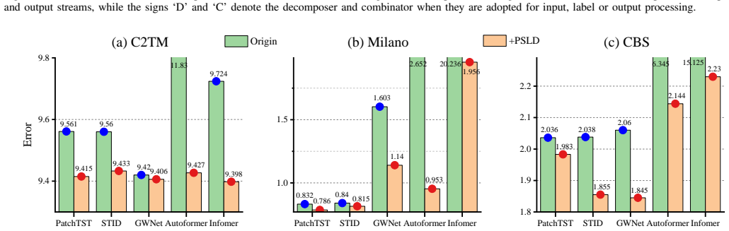
- The mechanism is not tied to the MLP backbone; adding PSLD-style supervision to PatchTST, STID, and GWNet improved their accuracy in the paper's experiments.
- The benefit generalizes beyond wireless traffic: PSLD also reports lower MSE than strong baselines on ETT, ILI, Weather, Electricity, and Traffic benchmarks.
Reading between the lines
- The label 'progressive' implies a curriculum, but the loss function sums all component losses from the start; whether ordering or gating component supervision would change results is an untested extension, and the framing predicts it should matter.
- Because the variance branch is trained to match the true spread of the series, it could be calibrated into a prediction interval; the paper notes this as future work rather than demonstrating it.
- The proof of Theorem 1 is referenced as Appendix II, but that appendix does not appear in the posted version; the unbiasedness claim should be read as asserted until the proof is available.
- RSS's unbiasedness is stated for aggregate features, not for edge-level topology; plugging graph-aware backbones into PSLD would reveal whether random node subgraphs preserve enough structure for spatial learning.
Editorial analysis
A structured set of objections, weighed in public.
Referee Report
Summary. The paper proposes PSLD (Progressive Supervision via Label Decomposition) for long-term, large-scale wireless traffic forecasting. It introduces Random Subgraph Sampling (RSS) to reduce the scale of graph-structured traffic data, decomposes the target label into mean/variance/residual or trend/seasonal/residual components, trains separate learner/predictor branches on each component, and recombines their outputs through a combinatory module. The authors report experiments on three wireless traffic datasets (C2TM, Milano, CBS) and several LTSF benchmarks, claiming average performance improvements of 2%, 4%, and 11% over existing methods, together with faster training and inference. They also release WTFlib, an open-source library for wireless traffic forecasting.
Significance. If the claims hold, the paper would offer a simple and computationally cheap way to improve long-term forecasting on non-stationary, large-scale traffic data, and RSS would provide a practical route to training on very large graphs. The paper has clear strengths: the decomposition/recombination equations are exact when the combinatory layer is an identity mapping; the authors release code and data links; and the efficiency comparison (Table IV) is a useful contribution. However, the central empirical claim of superiority over SOTA is not reproducible from the reported numbers, the theoretical statement for RSS lacks its proof, and the word 'progressive' is not backed by any progressive training mechanism. The significance of the contribution therefore cannot be assessed until these load-bearing issues are resolved.
major comments (4)
- [Abstract; Section IV.D, Table I] The claim of average 2%, 4%, and 11% improvement over SOTA is not reproducible from Table I. Averaging MSE over the reported horizons on C2TM gives 9.266 for PSLD-MVD versus 9.272 for the best baseline FreTS, a 0.06% gain; on Milano the PSLD-MVD average is 0.875 versus 0.912 for TimeMachine (4.0%); on CBS the PSLD-MVD average is 1.797 versus 1.887 for TimeMachine (4.8%), and the 11% figure is obtained only by comparing with PatchTST (2.026), which is not the strongest baseline on that dataset. Since no error bars or random seeds are reported, a 0.001 MSE difference at individual horizons (e.g., C2TM length-5, both 9.161) is not evidence of significant improvement. The headline claim therefore needs to be recomputed against the best baseline per dataset and accompanied by variance estimates.
- [Section II, Theorem 1 and Algorithm 1] Theorem 1 is the sole theoretical justification for RSS, but its proof is cited to 'Appendix II,' which is not present in the manuscript; the claim that sampled subgraphs are an unbiased estimator of true aggregate features is therefore unverifiable. Algorithm 1 also does not implement what the text describes: line 1 overwrites Nsub with Nnode/Nsub, and lines 7-8 index edge matrices by shuffled node indices without specifying how subgraphs are partitioned or selected, making the pseudocode incomplete.
- [Section III, Eq. (9), Fig. 3] The method is called 'progressive supervision,' but no progressive or curriculum mechanism is present. The component losses L_theta, L_phi, L_psi in Eq. (7) are summed with the combinatory loss in Eq. (9) from the first epoch with a fixed weight lambda; there is no staged training, no ordering of components by difficulty, and no schedule. The word 'progressively' in the description ('learned progressively at shallow layers') is not matched by any algorithmic step. To support the name and the claimed benefit of learning easy components first, the authors should compare against a non-progressive multi-task baseline that trains the same branches simultaneously with the same total loss.
- [Section IV.D, Table I (FourierGNN CBS row; PSLD-MVD C2TM MAE row)] The reported numbers contain anomalies that suggest unreviewed errors. For FourierGNN on CBS, MSE drops from 2.601 at length-24 to 1.193 at length-72, while most models degrade with horizon. For PSLD-MVD on C2TM, the MAE at length-7 is 0.317 while all other MAEs are about 0.17, yet the MSE at the same length is 9.431, consistent with the neighboring values. These entries need to be verified and corrected; if they are typographical errors, the table must be regenerated.
minor comments (7)
- [Title; Section IV.D] The title reads 'An Long-Term' and should be 'A Long-Term'; Section IV.D contains 'including including' in the sentence listing FreTS, TimeMachine, and FourierGNN.
- [Eq. (12) and Eq. (1)] The symbols M and S in Eq. (12) denote dataset mean and standard deviation, while Eq. (1) uses M and V for label component mean and variance; this notation conflict makes the preprocessing and decomposition steps harder to follow.
- [Table I caption] The caption says 'SIX BENCHMARK DATASETS' but the table reports results on three wireless traffic datasets; the caption should be corrected or clarified.
- [Section IV.B] The text states that batch size is set to 1 for large-scale graph WT datasets, but the interaction between RSS subgraph sampling and batching is not explained; it is unclear whether each batch is one subgraph or one time window across all subgraphs.
- [Table IV] The MSE column is reported without specifying the dataset and prediction setting; it appears to correspond to Milano input-36-predict-24, but this should be stated explicitly in the table or caption.
- [Fig. 1 caption] The caption mentions 'Flops (Bubble Size)' but gives no legend or numerical scale for bubble sizes, making the efficiency comparison difficult to interpret.
- [Abstract and Section I] WTFlib is described as an open-source library, but no formal citation, version number, or documentation reference is provided; the anonymous link contains a visible username, so the submission is not anonymized.
Circularity Check
No significant circularity: PSLD supervises components via a fixed deterministic label transform, and the final prediction uses predicted components rather than ground-truth labels.
full rationale
The derivation chain is self-contained in the relevant sense. In Section III.A, Eq. 1 defines the MVD components M, V, R as deterministic functions of the target variable Y. These are supervision targets, not fitted parameters. The learners and predictors in Eq. 4 map the decomposed input (M_X, V_X, R_X) to predicted components (\hat M, \hat V, \hat R). The combiner in Eq. 5 reconstructs the final forecast from those predicted components, not from the ground-truth M, V, R of the label (the notation 'V × R' in Eq. 5 is a typographical shorthand for the predicted components, since inference cannot access true label components). Thus the final prediction is not constructed from the labels by construction; it is a genuine function of the input. The component losses in Eq. 7 are auxiliary multi-task losses on transformed labels, while Eq. 8 ensures the final output matches Y. No parameter is fitted to a subset of the target and then renamed as a prediction. Self-citations are present: [47] (Periodformer) is used as a baseline, and [59] (Minusformer) is a same-author reference that does not appear to be cited in the running text. Neither is load-bearing for the central empirical claim. The proof of Theorem 1 is stated to be in 'Appendix II,' but the manuscript contains no Appendix II; this is an omitted proof and a completeness concern, not a circular reduction. Possible numerical discrepancies in Table I relative to the claimed 2%/4%/11% improvements are correctness risks, not circularity. Accordingly, no circular step is identified.
Assumptions & free parameters
free parameters (4)
- lambda (component loss weight) =
not reported
- kappa_T and kappa_S (STL smoothing kernel sizes) =
not reported
- epsilon (division-by-zero constant) =
not reported
- Nsub (number of subgraphs in RSS) =
24
assumptions (3)
- domain assumption RSS yields an unbiased estimator of the full graph's aggregate features.
- ad hoc to paper Decomposing the output label into mean, variance, and residual (or trend, seasonal, residual) produces components that are each easier to predict than the original series.
- ad hoc to paper Learning components at shallow layers and combining at deep layers (progressive supervision) improves accuracy without a curriculum.
Cite this review
Pith. "Pith review of Progressive Supervision via Label Decomposition: An Long-Term and Large-Scale Wireless Traffic Forecasting Method." pith.science (2026). https://pith.science/paper/RBCPZGAI
@misc{pith2026250106255,
  author       = {Pith},
  title        = {Pith review of: Progressive Supervision via Label Decomposition: An Long-Term and Large-Scale Wireless Traffic Forecasting Method},
  year         = {2026},
  howpublished = {\url{https://pith.science/paper/RBCPZGAI}},
  note         = {Machine review of arXiv:2501.06255}
}
read the original abstract
Long-term and Large-scale Wireless Traffic Forecasting (LL-WTF) is pivotal for strategic network management and comprehensive planning on a macro scale. However, LL-WTF poses greater challenges than short-term ones due to the pronounced non-stationarity of extended wireless traffic and the vast number of nodes distributed at the city scale. To cope with this, we propose a Progressive Supervision method based on Label Decomposition (PSLD). Specifically, we first introduce a Random Subgraph Sampling (RSS) algorithm designed to sample a tractable subset from large-scale traffic data, thereby enabling efficient network training. Then, PSLD employs label decomposition to obtain multiple easy-to-learn components, which are learned progressively at shallow layers and combined at deep layers to effectively cope with the non-stationary problem raised by LL-WTF tasks. Finally, we compare the proposed method with various state-of-the-art (SOTA) methods on three large-scale WT datasets. Extensive experimental results demonstrate that the proposed PSLD significantly outperforms existing methods, with an average 2%, 4%, and 11% performance improvement on three WT datasets, respectively. In addition, we built an open source library for WT forecasting (WTFlib) to facilitate related research, which contains numerous SOTA methods and provides a strong benchmark.Experiments can be reproduced through https://github.com/Anoise/WTFlib.
Figures


Figures from the paper (7 more)






Reference graph
Works this paper leans on
-
[1]
Cisco annual internet report (2018–2023) white paper,
U. Cisco, “Cisco annual internet report (2018–2023) white paper,” Cisco: San Jose, CA, USA , vol. 10, no. 1, pp. 1–35, 2020
2018
-
[2]
A variegated look at 5g in the wild: performance, power, and qoe implications,
A. Narayanan, X. Zhang, R. Zhu, A. Hassan, S. Jin, X. Zhu, X. Zhang, D. Rybkin, Z. Yang, Z. M. Mao et al., “A variegated look at 5g in the wild: performance, power, and qoe implications,” in Proceedings of the 2021 ACM SIGCOMM 2021 Conference , 2021, pp. 610–625
2021
-
[3]
Evolution of wireless communication to 6g: Potential applications and research directions,
M. Z. Asghar, S. A. Memon, and J. H ¨am¨al¨ainen, “Evolution of wireless communication to 6g: Potential applications and research directions,” Sustainability, vol. 14, no. 10, p. 6356, 2022
work page 2022
-
[4]
Cell zooming for cost-efficient green cellular networks,
Z. Niu, Y . Wu, J. Gong, and Z. Yang, “Cell zooming for cost-efficient green cellular networks,” IEEE communications magazine , vol. 48, no. 11, pp. 74–79, 2010
work page 2010
-
[5]
N. Kato, Z. M. Fadlullah, B. Mao, F. Tang, O. Akashi, T. Inoue, and K. Mizutani, “The deep learning vision for heterogeneous network traffic control: Proposal, challenges, and future perspective,” IEEE wireless communications, vol. 24, no. 3, pp. 146–153, 2016
work page 2016
-
[6]
Deepcog: Optimizing resource provisioning in network slicing with ai-based capacity forecasting,
D. Bega, M. Gramaglia, M. Fiore, A. Banchs, and X. Costa-P ´erez, “Deepcog: Optimizing resource provisioning in network slicing with ai-based capacity forecasting,” IEEE Journal on Selected Areas in Communications, vol. 38, no. 2, pp. 361–376, 2020
work page 2020
-
[7]
Intelligent 5g: When cellular networks meet artificial intelligence,
R. Li, Z. Zhao, X. Zhou, G. Ding, Y . Chen, Z. Wang, and H. Zhang, “Intelligent 5g: When cellular networks meet artificial intelligence,” IEEE Wireless communications, vol. 24, no. 5, pp. 175–183, 2017
work page 2017
-
[8]
Wireless traffic modeling and prediction using seasonal arima models,
Y . Shu, M. Yu, O. Yang, J. Liu, and H. Feng, “Wireless traffic modeling and prediction using seasonal arima models,” IEICE transactions on communications, vol. 88, no. 10, pp. 3992–3999, 2005
work page 2005
Show all 64 references
-
[9]
Traffic predictability based on arima/garch model,
B. Zhou, D. He, and Z. Sun, “Traffic predictability based on arima/garch model,” in 2006 2nd Conference on Next Generation Internet Design and Engineering, 2006. NGI’06. IEEE, 2006, pp. 200–207
2006
-
[10]
Big data driven mobile traffic understanding and forecasting: A time series approach,
F. Xu, Y . Lin, J. Huang, D. Wu, H. Shi, J. Song, and Y . Li, “Big data driven mobile traffic understanding and forecasting: A time series approach,” IEEE transactions on services computing , vol. 9, no. 5, pp. 796–805, 2016
2016
-
[11]
The prediction analysis of cellular radio access network traffic: From entropy theory to networking practice,
R. Li, Z. Zhao, X. Zhou, J. Palicot, and H. Zhang, “The prediction analysis of cellular radio access network traffic: From entropy theory to networking practice,” IEEE Communications Magazine , vol. 52, no. 6, pp. 234–240, 2014
2014
-
[12]
Analyzing and modeling spatio-temporal dependence of cellular traffic at city scale,
X. Chen, Y . Jin, S. Qiang, W. Hu, and K. Jiang, “Analyzing and modeling spatio-temporal dependence of cellular traffic at city scale,” in 2015 IEEE international conference on communications (ICC) . IEEE, 2015, pp. 3585–3591
2015
-
[13]
The learning and prediction of application-level traffic data in cellular networks,
R. Li, Z. Zhao, J. Zheng, C. Mei, Y . Cai, and H. Zhang, “The learning and prediction of application-level traffic data in cellular networks,” IEEE Transactions on Wireless Communications , vol. 16, no. 6, pp. 3899–3912, 2017
2017
-
[14]
25 years of time series forecast- ing,
J. G. De Gooijer and R. J. Hyndman, “25 years of time series forecast- ing,” International journal of forecasting , vol. 22, no. 3, pp. 443–473, 2006
2006
-
[15]
A study of deep learning networks on mobile traffic forecasting,
C.-W. Huang, C.-T. Chiang, and Q. Li, “A study of deep learning networks on mobile traffic forecasting,” in 2017 IEEE 28th annual international symposium on personal, indoor, and mobile radio com- munications (PIMRC), 2017, pp. 1–6
2017
-
[16]
Citywide cellular traffic prediction based on densely connected convolutional neural networks,
C. Zhang, H. Zhang, D. Yuan, and M. Zhang, “Citywide cellular traffic prediction based on densely connected convolutional neural networks,” IEEE Communications Letters , vol. 22, no. 8, pp. 1656–1659, 2018
2018
-
[17]
Deep transfer learning for intelligent cellular traffic prediction based on cross-domain big data,
C. Zhang, H. Zhang, J. Qiao, D. Yuan, and M. Zhang, “Deep transfer learning for intelligent cellular traffic prediction based on cross-domain big data,” IEEE Journal on Selected Areas in Communications , vol. 37, no. 6, pp. 1389–1401, 2019
2019
-
[18]
Mvstgn: A multi-view spatial- temporal graph network for cellular traffic prediction,
Y . Yao, B. Gu, Z. Su, and M. Guizani, “Mvstgn: A multi-view spatial- temporal graph network for cellular traffic prediction,” IEEE Transac- tions on Mobile Computing , 2021
2021
-
[19]
Dynamic graph convolutional recurrent network for traffic prediction: Benchmark and solution,
F. Li, J. Feng, H. Yan, G. Jin, F. Yang, F. Sun, D. Jin, and Y . Li, “Dynamic graph convolutional recurrent network for traffic prediction: Benchmark and solution,” ACM Transactions on Knowledge Discovery from Data, vol. 17, no. 1, pp. 1–21, 2023
2023
-
[20]
Approximation capabilities of multilayer feedforward net- works,
K. Hornik, “Approximation capabilities of multilayer feedforward net- works,” Neural networks, vol. 4, no. 2, pp. 251–257, 1991
1991
-
[21]
Gradient-based learning applied to document recognition,
Y . LeCun, L. Bottou, Y . Bengio, and P. Haffner, “Gradient-based learning applied to document recognition,” Proceedings of the IEEE , vol. 86, no. 11, pp. 2278–2324, 1998
1998
-
[22]
The graph neural network model,
F. Scarselli, M. Gori, A. C. Tsoi, M. Hagenbuchner, and G. Monfar- dini, “The graph neural network model,” IEEE transactions on neural networks, vol. 20, no. 1, pp. 61–80, 2008
2008
-
[23]
Recurrent neural net- works and robust time series prediction,
J. T. Connor, R. D. Martin, and L. E. Atlas, “Recurrent neural net- works and robust time series prediction,” IEEE Transactions on Neural Networks, vol. 5, no. 2, pp. 240–254, 1994
1994
-
[24]
A meta-learning scheme for adaptive short-term network traffic prediction,
Q. He, A. Moayyedi, G. D ´an, G. P. Koudouridis, and P. Tengkvist, “A meta-learning scheme for adaptive short-term network traffic prediction,” IEEE Journal on Selected Areas in Communications, vol. 38, no. 10, pp. 2271–2283, 2020
2020
-
[25]
A forecasting approach to improve control and management for 5g networks,
D. Ferreira, A. Braga Reis, C. Senna, and S. Sargento, “A forecasting approach to improve control and management for 5g networks,” IEEE Transactions on Network and Service Management , vol. 18, no. 2, pp. 1817–1831, 2021
2021
-
[26]
Context- aware traffic prediction: Loss function formulation for predicting traffic in 5g networks,
L. A. Garrido, P.-V . Mekikis, A. Dalgkitsis, and C. Verikoukis, “Context- aware traffic prediction: Loss function formulation for predicting traffic in 5g networks,” in ICC 2021 - IEEE International Conference on Communications, 2021, pp. 1–6
2021
-
[27]
Mobile traffic forecasting using a combined fft/lstm strategy in sdn networks,
M. L. Hachemi, A. Ghomari, Y . Hadjadj-Aoul, and G. Rubino, “Mobile traffic forecasting using a combined fft/lstm strategy in sdn networks,” in 2021 IEEE 22nd International Conference on High Performance Switching and Routing (HPSR) . IEEE, 2021, pp. 1–6
2021
-
[28]
Forecasting at scale,
S. J. Taylor and B. Letham, “Forecasting at scale,” The American Statistician, vol. 72, no. 1, pp. 37–45, 2018
2018
-
[29]
N-beats: Neural basis expansion analysis for interpretable time series forecasting,
B. N. Oreshkin, D. Carpov, N. Chapados, and Y . Bengio, “N-beats: Neural basis expansion analysis for interpretable time series forecasting,” in International Conference on Learning Representations , 2019
2019
-
[30]
Think globally, act locally: A deep neural network approach to high-dimensional time series forecasting,
R. Sen, H.-F. Yu, and I. S. Dhillon, “Think globally, act locally: A deep neural network approach to high-dimensional time series forecasting,” Advances in neural information processing systems , vol. 32, 2019
2019
-
[31]
Autoformer: Decomposition transformers with auto-correlation for long-term series forecasting,
H. Wu, J. Xu, J. Wang, and M. Long, “Autoformer: Decomposition transformers with auto-correlation for long-term series forecasting,” in Advances in Neural Information Processing Systems (NeurIPS) , vol. 34, Virtual Conference, 2021, pp. 22 419–22 430
2021
-
[32]
FED- former: Frequency enhanced decomposed transformer for long-term series forecasting,
T. Zhou, Z. Ma, Q. Wen, X. Wang, L. Sun, and R. Jin, “FED- former: Frequency enhanced decomposed transformer for long-term series forecasting,” in Proceedings of the 39th International Conference on Machine Learning (ICML), vol. 162, Baltimore, Maryland, 2022, pp. 27 268–27 286
2022
-
[33]
Non-stationary transformers: Exploring the stationarity in time series forecasting,
Y . Liu, H. Wu, J. Wang, and M. Long, “Non-stationary transformers: Exploring the stationarity in time series forecasting,” Advances in Neural Information Processing Systems , vol. 35, pp. 9881–9893, 2022
2022
-
[34]
Progressive neural networks,
A. A. Rusu, N. C. Rabinowitz, G. Desjardins, H. Soyer, J. Kirkpatrick, K. Kavukcuoglu, R. Pascanu, and R. Hadsell, “Progressive neural networks,” arXiv preprint arXiv:1606.04671 , 2016
2016 arXiv
-
[35]
Stl: A seasonal-trend decomposition,
R. B. Cleveland, W. S. Cleveland, J. E. McRae, and I. Terpenning, “Stl: A seasonal-trend decomposition,” J. Off. Stat , vol. 6, no. 1, pp. 3–73, 1990
1990
-
[36]
Forecasting time series with complex seasonal patterns using exponential smoothing,
A. M. De Livera, R. J. Hyndman, and R. D. Snyder, “Forecasting time series with complex seasonal patterns using exponential smoothing,” Journal of the American statistical association , vol. 106, no. 496, pp. 1513–1527, 2011
2011
-
[37]
Time series forecasting for nonlinear and non- stationary processes: a review and comparative study,
C. Cheng, A. Sa-Ngasoongsong, O. Beyca, T. Le, H. Yang, Z. Kong, and S. T. Bukkapatnam, “Time series forecasting for nonlinear and non- stationary processes: a review and comparative study,” Iie Transactions, vol. 47, no. 10, pp. 1053–1071, 2015
2015
-
[38]
Analyzing and modeling spatio-temporal dependence of cellular traffic at city scale,
Y . J. Xiaming Chen, S. Qiang, W. Hu, and K. Jiang, “Analyzing and modeling spatio-temporal dependence of cellular traffic at city scale,” in Communications (ICC), 2015 IEEE International Conference on , 2015
2015
-
[39]
A multi-source dataset of urban life in the city of milan and the province of trentino,
G. Barlacchi, M. De Nadai, R. Larcher, A. Casella, C. Chitic, G. Torrisi, F. Antonelli, A. Vespignani, A. Pentland, and B. Lepri, “A multi-source dataset of urban life in the city of milan and the province of trentino,” Scientific data, vol. 2, no. 1, pp. 1–15, 2015
2015
-
[40]
Adam: A method for stochastic optimiza- tion,
D. P. Kingma and J. Ba, “Adam: A method for stochastic optimiza- tion,” in International Conference on Learning Representations (ICLR) , Santiago de Cuba, 2015
2015
-
[41]
Informer: Beyond efficient transformer for long sequence time-series forecasting,
H. Zhou, S. Zhang, J. Peng, S. Zhang, J. Li, H. Xiong, and W. Zhang, “Informer: Beyond efficient transformer for long sequence time-series forecasting,” in Proceedings of the 35th AAAI Conference on Artificial Intelligence (AAAI) , vol. 35, no. 12, Virtual Conference, 2021, pp...
2021
-
[42]
Frequency-domain mlps are more effective learners in time series forecasting,
K. Yi, Q. Zhang, W. Fan, S. Wang, P. Wang, H. He, N. An, D. Lian, L. Cao, and Z. Niu, “Frequency-domain mlps are more effective learners in time series forecasting,” Advances in Neural Information Processing Systems, vol. 36, 2024
2024
-
[43]
Timemachine: A time series is worth 4 mambas for long-term forecasting,
M. A. Ahamed and Q. Cheng, “Timemachine: A time series is worth 4 mambas for long-term forecasting,” arXiv preprint arXiv:2403.09898, 2024
2024 arXiv
-
[44]
Fouriergnn: Rethinking multivariate time series forecast- ing from a pure graph perspective,
K. Yi, Q. Zhang, W. Fan, H. He, L. Hu, P. Wang, N. An, L. Cao, and Z. Niu, “Fouriergnn: Rethinking multivariate time series forecast- ing from a pure graph perspective,” Advances in Neural Information Processing Systems, vol. 36, 2024
2024
-
[45]
A time series is worth 64 words: Long-term forecasting with transformers,
Y . Nie, N. H. Nguyen, P. Sinthong, and J. Kalagnanam, “A time series is worth 64 words: Long-term forecasting with transformers,” in The Eleventh International Conference on Learning Representations , 2023
2023
-
[46]
Spatial-temporal identity: A simple yet effective baseline for multivariate time series forecasting,
Z. Shao, Z. Zhang, F. Wang, W. Wei, and Y . Xu, “Spatial-temporal identity: A simple yet effective baseline for multivariate time series forecasting,” in Proceedings of the 31st ACM International Conference on Information & Knowledge Management , 2022, pp. 4454–4458
2022
-
[47]
Does long- term series forecasting need complex attention and extra long inputs?
D. Liang, H. Zhang, D. Yuan, X. Ma, D. Li, and M. Zhang, “Does long- term series forecasting need complex attention and extra long inputs?” arXiv preprint arXiv:2306.05035 , 2023
2023 arXiv
-
[48]
Are transformers effective for time series forecasting?
A. Zeng, M. Chen, L. Zhang, and Q. Xu, “Are transformers effective for time series forecasting?” in Proceedings of the AAAI conference on artificial intelligence, vol. 37, no. 9, 2023, pp. 11 121–11 128
2023
-
[49]
Attention is all you need,
A. Vaswani, N. Shazeer, N. Parmar, J. Uszkoreit, L. Jones, A. N. Gomez, L. u. Kaiser, and I. Polosukhin, “Attention is all you need,” in Advances in 31st Neural Information Processing Systems (NeurIPS), vol. 30, Long Beach, USA, 2017, pp. 6000–6010
2017
-
[50]
Graph wavenet for deep spatial-temporal graph modeling,
Z. Wu, S. Pan, G. Long, J. Jiang, and C. Zhang, “Graph wavenet for deep spatial-temporal graph modeling,” in Proceedings of the Twenty-Eighth International Joint Conference on Artificial Intelligence . International Joint Conferences on Artificial Intelligence Organization, 2019
2019
-
[51]
A distance measure for classifying arima models,
D. Piccolo, “A distance measure for classifying arima models,” Journal of time series analysis , vol. 11, no. 2, pp. 153–164, 1990
1990
-
[52]
Exponential smoothing: The state of the art,
E. S. Gardner Jr, “Exponential smoothing: The state of the art,” Journal of forecasting, vol. 4, no. 1, pp. 1–28, 1985
1985
-
[53]
Parsimonious linear fingerprint- ing for time series,
L. Li, B. A. Prakash, and C. Faloutsos, “Parsimonious linear fingerprint- ing for time series,” Proceedings of the VLDB Endowment , vol. 3, no. 1-2, pp. 385–396, 2010
2010
-
[54]
Classification and regression by randomfor- est,
A. Liaw, M. Wiener et al., “Classification and regression by randomfor- est,” R News, vol. 2, no. 3, pp. 18–22, 2002
2002
-
[55]
Online-svr for short-term traffic flow prediction under typical and atypical traffic conditions,
M. Castro-Neto, Y .-S. Jeong, M.-K. Jeong, and L. D. Han, “Online-svr for short-term traffic flow prediction under typical and atypical traffic conditions,” Expert Systems with Applications , vol. 36, no. 3, pp. 6164– 6173, 2009
2009
-
[56]
Densely connected convolutional networks,
G. Huang, Z. Liu, L. Van Der Maaten, and K. Q. Weinberger, “Densely connected convolutional networks,” in Proceedings of the IEEE Confer- ence on Computer Vision and Pattern Recognition, 2017, pp. 4700–4708
2017
-
[57]
Difftad: Denoising diffusion probabilistic models for vehicle trajectory anomaly detection,
C. Li, G. Feng, Y . Li, R. Liu, Q. Miao, and L. Chang, “Difftad: Denoising diffusion probabilistic models for vehicle trajectory anomaly detection,” Knowledge-Based Systems, vol. 286, p. 111387, 2024
2024
-
[58]
A time series is worth 64 words: Long-term forecasting with transformers,
Y . Nie, N. H. Nguyen, P. Sinthong, and J. Kalagnanam, “A time series is worth 64 words: Long-term forecasting with transformers,” in The Eleventh International Conference on Learning Representations , 2022
2022
-
[59]
Minusformer: Improving time series forecasting by progressively learning residuals,
D. Liang, H. Zhang, D. Yuan, B. Zhang, and M. Zhang, “Minusformer: Improving time series forecasting by progressively learning residuals,” arXiv preprint arXiv:2402.02332 , 2024
2024 arXiv
-
[60]
En- hancing the locality and breaking the memory bottleneck of transformer on time series forecasting,
S. Li, X. Jin, Y . Xuan, X. Zhou, W. Chen, Y .-X. Wang, and X. Yan, “En- hancing the locality and breaking the memory bottleneck of transformer on time series forecasting,” in Advances in 33rd Neural Information Processing Systems (NeurIPS) , vol. 32, Vancouver, Canada, 2019, ...
2019
-
[61]
Time-series,
O. D. Anderson, “Time-series,” Journal of the Royal Statistical Society. Series D (The Statistician) , vol. 25, no. 4, pp. 308–310, 1976
1976
-
[62]
Stwave ++: A multi- scale efficient spectral graph attention network with long-term trends for disentangled traffic flow forecasting,
Y . Fang, Y . Qin, H. Luo, F. Zhao, and K. Zheng, “Stwave ++: A multi- scale efficient spectral graph attention network with long-term trends for disentangled traffic flow forecasting,” IEEE Transactions on Knowledge and Data Engineering , vol. 36, no. 6, pp. 2671–2685, 2024
2024
-
[63]
When spatio-temporal meet wavelets: Disentangled traffic forecasting via efficient spectral graph attention networks,
Y . Fang, Y . Qin, H. Luo, F. Zhao, B. Xu, L. Zeng, and C. Wang, “When spatio-temporal meet wavelets: Disentangled traffic forecasting via efficient spectral graph attention networks,” in 2023 IEEE 39th International Conference on Data Engineering (ICDE) , 2023, pp. 517– 529
2023
-
[64]
Spatio-temporal hierarchical mlp network for traffic forecasting,
Y . Qin, H. Luo, F. Zhao, Y . Fang, X. Tao, and C. Wang, “Spatio-temporal hierarchical mlp network for traffic forecasting,” Information Sciences, vol. 632, pp. 543–554, 2023
2023
Reviewed August 10, 2026 · model on record in the stance chip above.
Discussion (0). Continue with ORCID to comment.