REVIEW 4 major objections 8 minor 33 references
Reconstructing Time-of-Flight Detector Values of Angular Streaking Using Machine Learning
T0 review · 4 major / 8 minor · reviewed 2026-08-10 · deepseek-v4-flash
Pith's one-line read The paper claims that a convolutional autoencoder trained only on simulated time-of-flight detector images can denoise angular-streaking data and reconstruct up to three failed detectors in a 16-detector array, fast enough for online use…
desk verdict A solid, well-evaluated ML tool for TOF detector denoising and reconstruction; the sim-to-real transfer is the main soft spot, and an off-by-one bug in the disablement algorithm needs fixing. read the letter →
The pith
A machine-rendered reading of the paper's core claim, the machinery that carries it, and where it could break.
The reading
What carries the argument
The load-bearing mechanism is a partial-wave simulation of the streaking process that turns random spectrograms into detector images via $d_{ij} = \sum_{i,j} \mathrm{sim}(j,\kappa,2\pi i/80) s_{ij}$, with measured polarisation ellipticity $\varepsilon=0.73$, tilt $\theta=3\pi/8$, anisotropy $\beta_2=2$, and kick $\kappa\sim U(0,100)\,\mathrm{eV}$. Around this simulation the paper builds an end-to-end training corruption: min-max normalization, additive Gaussian noise with $\sigma\sim U(0,0.2)$, random single-pixel hot spots, and one to three TOF detectors zeroed out, with the clean simulation as the target. The network itself is a convolutional autoencoder with a bottleneck of 64 filters; the bottleneck is what forces the model to learn the global angular correlation pattern, so that a zeroed channel is reconstructed from the other 15 rather than from local averaging alone. The General model is the version trained with one to three random failures, and the paper's comparisons to specialized models and to the mean model isolate the contribution of this learned redundancy.
What would settle it
During a real LCLS run, deliberately disable one healthy TOF detector, apply the General model to the remaining 15 channels, and compare the reconstructed channel with the measured values from the disabled detector; matching the simulated RMSE of about $2.5\times10^{-3}$ (normalized intensity) would confirm the simulation-to-real transfer, while errors orders of magnitude larger would refute it.
Extended reading notes
Core claim
The central claim, stated on the paper's own terms, is that the information lost when a TOF detector fails is redundant across the remaining 15 channels, and that this redundancy is learnable from simulation alone. A single convolutional autoencoder with a 64-filter bottleneck, trained on millions of simulated 16×60 detector images corrupted by Gaussian noise, hot-pixel spikes, and zeroed channels, maps noisy and incomplete inputs back to clean, complete images. On the simulated test set the General model reaches RMSE $2.48\times10^{-3}$ for one failed detector, $2.64\times10^{-3}$ for two, and $2.86\times10^{-3}$ for three, roughly 30 times better than the neighbor-averaging baseline, and a deliberately specialized model does even better when the failed positions are known in advance. On real LCLS data the paper demonstrates the same behaviour visually: denoised images resemble the originals, and reconstructions of disabled detectors blend in with the full image. The paper is explicit that a numerical evaluation on real-world images is impossible because noiseless ground-truth detector images do not exist.
Load-bearing premise
Everything rests on the assumption that the simulated detector images, corrupted with Gaussian noise, hot pixels, and zeroed channels, are realistic enough that a network trained only on those simulations keeps its accuracy on the real LCLS detector; the paper itself says no quantitative real-world comparison is possible.
Editorial extensions
If this is right
- At LCLS, where data arrive at 120 detector images per second, the method's 217.53 ms processing time for 1024 images means denoising and reconstruction can run inside the one-second inter-batch interval, enabling live monitoring.
- Up to three failed detectors can be filled in during the experiment, so runs with partial detector failure no longer have to be discarded or reconstructed only offline.
- The General model is the safest choice when failures are unpredictable; a model trained for specific positions does better only when the failed positions are known in advance.
- Reconstruction error rises with the number of failures and degrades noticeably at four or five detectors, bounding the method's operational range.
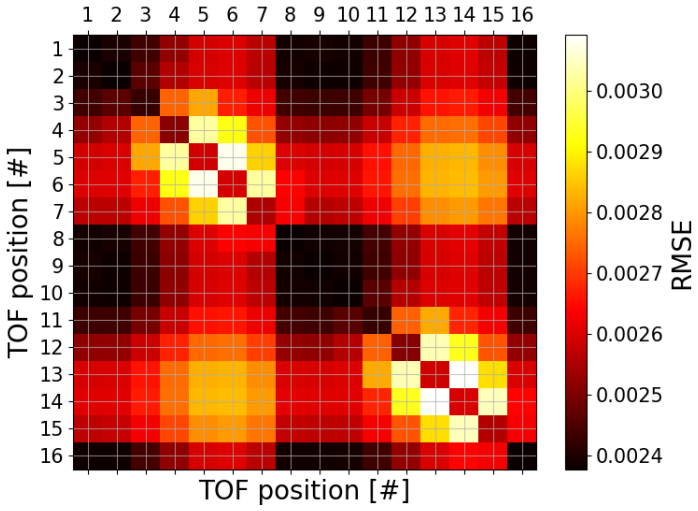
- Error maps across detector positions identify which channels carry redundant information, giving a quantitative basis for redesigning the TOF array geometry.
Reading between the lines
- If the simulation-to-real transfer is as good as the visual results suggest, the same pipeline could be retargeted to other spectrometer geometries simply by regenerating synthetic data, turning the trained network into a reusable instrument-design tool.
- A direct real-world test is easy to run but is not reported: disable one healthy detector on live data and compare the model output with the measured values from that detector; the paper's real-world evidence is currently qualitative only.
- The pair-error matrix suggests a design heuristic: avoid placing high-intensity detectors in correlated failure groups, since those pairs produce the worst reconstructions, and this layout principle is testable in simulation.
- Because the paper explicitly leaves detector-failure detection to future work, coupling this reconstructor with an online anomaly detector would complete an autonomous pipeline that both notices and repairs failed channels.
Editorial analysis
A structured set of objections, weighed in public.
Referee Report
Summary. The paper proposes a convolutional-autoencoder-based method to denoise and reconstruct up to three failed time-of-flight (TOF) detectors in angular streaking experiments. The network is trained exclusively on simulated detector images augmented with Gaussian noise, random hot pixels, and disabled detectors; several bottleneck sizes and training variants (1TOF, 2TOF, 3TOF, General, Spec) are compared against a neighbor-averaging baseline on a large simulated test set. The authors also show qualitative results on real LCLS data and report inference timing that supports online use during an experiment.
Significance. If the simulation-to-real transfer holds, the method is practically valuable: it offers a fast, code-released denoising and reconstruction tool for a running experiment, with a meaningful comparison against a simple baseline and a large synthetic evaluation that includes confidence intervals. The main strength is the thorough simulated benchmark, the public code, and the design-oriented observation about which TOF positions are harder to reconstruct. However, the real-world validation is visual only, and the noise and failure model parameters are not measured from real detector statistics, so the central claim of real-world applicability currently rests on an unquantified transfer assumption.
major comments (4)
- [Sec. V] The statement that "A numerical evaluation for real-world images is impossible since we cannot generate noiseless detector images for comparison" is correct for denoising but not for reconstruction. On real data with functioning detectors, one can artificially disable a detector and compare the network's prediction for that detector to the actually recorded values. This leave-one-detector-out test should be added; without it, the paper's real-world reconstruction claim is supported only by visual inspection, which is not sufficient for the quantitative performance claimed in the abstract.
- [Sec. III A and Sec. IV A / Fig. 3] The test-set size is inconsistent: Sec. III A states "we limited the test data to 100000 samples," while Sec. IV A refers to "the large test sample size of 600000" and Fig. 3's caption says "600000 simulated examples." This contradiction affects the confidence-interval calculations and the statistical-significance discussion, so the authors should give the exact test-set size and recompute the reported statistics if necessary.
- [Appendix C, Algorithm 1] Algorithm 1 has an apparent off-by-one issue: after initializing ldisabled with one element, it draws ndisabled ~ U(0, nmax) and then runs the loop "for i in {0, ..., ndisabled}," which executes ndisabled+1 times. The effective number of disabled detectors can therefore exceed the advertised maximum nmax; for nmax=3, the General model's training distribution can include up to five disabled detectors. This makes the "up to three failed detectors" claim imprecise and the training distribution ambiguous, so the loop range or the sampling procedure should be corrected and the experiments rerun or justified.
- [Sec. III B] The noise model parameters are selected by visual similarity rather than measured from real detector statistics: the text says the parameters are chosen "so that the noised images look as similar as possible to the real images" and that the simulated noise level is "visually higher" than real noise. Because the network is trained only on this simulated noise, the reported RMSE values (e.g., 2.48e-3 for the General model in Tab. V) may not transfer if the actual detector noise, hot-pixel statistics, or failure patterns differ. A sensitivity analysis varying sigma, ppeak, and gamma around the chosen values, or a quantitative comparison of simulated and real noise statistics, would materially reduce this risk.
minor comments (8)
- [Sec. III B, Eq. (8)] The conditional expression in Eq. (8) is inconsistent with the preceding sentence: the sentence says a pixel is set to the maximum when p_ij <= p_peak, but the equation sets it to x_ij in that case and to the maximum otherwise. The branches should be swapped.
- [Sec. III C] The learning rate is reported as "eta = 10^4," which is presumably a typo for 10^-4; this should be corrected.
- [Sec. IV A and Fig. 5] The text says Fig. 5 shows a comparison using "the model only trained on the scenario of failed TOF detectors #8 and #13," but the caption states that all models in Fig. 5 are trained in the general setting. The text or the figure caption should be aligned.
- [Sec. V and Tab. VIII] The sentence "We also tested the previously described CCNNs, which even decreased the reconstruction error" is not supported by Tab. VIII, where the CCNN values are slightly higher than the CAE-64 baseline (e.g., 2.49e-3 vs. 2.48e-3 for one failed TOF). The claim should be rephrased or the data corrected.
- [Sec. IV A] The explanation of the confidence intervals is confusing: the text first says "CIs of the means" and then refers to "the CIs of this difference." The bracketed values in the tables should be explicitly defined as confidence intervals for the difference from the best model, or the wording should be made consistent.
- [Abstract and Introduction] The phrase "enable for experimentation in the attosecond regions" is ungrammatical; consider "enable experimentation in the attosecond regime." Similar wording issues appear in the Introduction.
- [Sec. V] The sentence "A higher value in the angular distribution ... means these areas often have lower intensities" is confusing: according to Eq. (4), a higher I_electron corresponds to higher intensity, so the relationship described should be clarified or rephrased.
- [Tab. III and Sec. IV A] For the zero-failed-detector scenario, the Mean model's output is not defined: with no detector disabled, it is unclear what the model averages. The definition of the baseline for this scenario should be stated.
Circularity Check
No circular derivation: the supervised targets are independent simulated images; real-world validation is visual only, which is a sim-to-real gap rather than a constructional circularity.
full rationale
I find no circular step that satisfies the evidentiary bar. The neural networks are trained to map simulated noisy/incomplete detector images to the same simulation's clean, complete images; the held-out simulated test RMSE (Tabs. III-V) is an independent benchmark of that supervised task, and the mean-model and Wiener-filter baselines provide external comparisons. The real-world application in Sec. V is explicitly not quantitatively evaluated ('A numerical evaluation for real-world images is impossible since we cannot generate noiseless detector images for comparison'), and the visual check is weakened by the fact that the synthetic noise parameters were chosen 'so that the noised images look as similar as possible to the real images' (Sec. III B). That is a generalization/validation gap, not a case where the prediction is defined in terms of the fitted inputs. The load-bearing simulation is the authors' own prior work ('partial-wave-based simulation by Hartmann et al.'), but it is publicly available code, its equations are stated in Sec. III A, and the cited paper [3] anchors it to real LCLS data; per the hard rules, such code-reproduced, externally falsifiable support does not constitute circularity. A separate off-by-one in Algorithm 1 (ndisabled ~ U(0,nmax) with a loop over 0..ndisabled) makes the effective number of disabled detectors exceed the advertised maximum, but this is a reproducibility/implementation concern outside circularity. Score 2 reflects the minor self-citation and the untested sim-to-real assumption, not a constructional reduction.
Assumptions & free parameters
free parameters (6)
- Gaussian noise sigma range =
sigma ~ U(0, 0.2)
- Hot-pixel probability ppeak =
not stated in text
- Neighbor/opposite disablement probability gamma =
0.5
- Kick parameter distribution =
U(0, 100) eV
- Spectrogram peak count and width =
1-5 peaks, sigma_max = 7 phase steps
- Gaussian width sigma_E for partial waves =
1 eV
assumptions (5)
- domain assumption The partial-wave simulation (Eqs. 1-6) accurately describes the real angular streaking detector response for this experiment.
- domain assumption Real detector noise can be approximated by additive Gaussian noise with random variance and random high-intensity spikes.
- domain assumption Failed TOF detectors produce zero values in all channels.
- domain assumption Mapping to 1 eV energy bins and redistributing empty bins from neighbors preserves the relevant signal.
- domain assumption Per-image min-max normalization loses no essential information for downstream pulse characterization.
Cite this review
Pith. "Pith review of Reconstructing Time-of-Flight Detector Values of Angular Streaking Using Machine Learning." pith.science (2026). https://pith.science/paper/3AYKM3E4
@misc{pith2026250108966,
  author       = {Pith},
  title        = {Pith review of: Reconstructing Time-of-Flight Detector Values of Angular Streaking Using Machine Learning},
  year         = {2026},
  howpublished = {\url{https://pith.science/paper/3AYKM3E4}},
  note         = {Machine review of arXiv:2501.08966}
}
read the original abstract
Angular streaking experiments enable for experimentation in the attosecond regions. However, the deployed Time-of-flight detectors are susceptible to noise and failure. These shortcomings make the outputs of the Time-of-flight detectors hard to understand for humans and further processing, such as for example the extraction of beam properties. In this article, we present an approach to remove high noise levels and reconstruct up to three failed Time-of-flight detectors from an arrangement of 16 Time-of-flight detectors. Due to its fast evaluation time, the presented method is applicable online during a running experiment. It is trained with simulation data, and we show the results of denoising and reconstruction of our method on real-world experiment data.
Figures


Figures from the paper (6 more)


Reference graph
Works this paper leans on
-
[1]
The intensity of these pixels is also random, uniformly distributed
Dataset High-Intensity Peaks: During dataset creation, we simulate 1-15 random single pixels of high intensity by adding random, uniformly distributed single pixel spots to the spectrogram. The intensity of these pixels is also random, uniformly distributed. These peaks create isolated, high-intensity spots in the detector images, mimicking spikes as show...
-
[2]
We choose the maximum value, so that it imitates a high intensity noise peak
Training High-Intensity Peaks: To create this noise, we set a probabilityppeak to which every pixel of a TOF detector is set to the maximum value of the detector image. We choose the maximum value, so that it imitates a high intensity noise peak. In a later step, we add Gaussian noise to the entire detector image, so that the Gaussian noise is also applie...
-
[3]
We apply the normalization individually per image
Normalization: Next, we min-max normalize the detector images. We apply the normalization individually per image. The real-world images are also normalized per 11 Model Training Data 1TOF, 2TOF, 3TOF Disable 1, 2 or 3 random TOF detectors respectively General Disable 1–3 TOF detectors randomly Spec Disable the TOF detectors at positions #8 and #13 Mean No...
-
[4]
Gaussian Noise: It is important that the previous normalization step is performed first, ensuring that the Gaussian noise is added to the normalized values, as illustrated in the following equation: ˜xij = ¯xij + pij (9) The variablesi and j are chosen similar to Eq. (7). The entries of the random matrix P are drawn from a Gaussian distribution: pij ∼ N 0...
-
[5]
Detector disablement: The next step is to disable the TOF detectors, with specific methods applied for training each model, as listed in Tab. II. In the following, ’#’ denotes a TOF detector’s position, while a number before TOF detectors indicates the count of uniformly random-selected TOF detectors. The selection strategy of which TOF detectors to disab...
-
[6]
Normalization: Min-max normalization is applied to each image individually again, ensuring that the values of the detector images—captured with disabled TOF 12 detectors—are rescaled between zero and one. This normalization process can also be implemented in real-world scenarios where TOF detector failures occur. This ap- proach remains valid since we foc...
-
[7]
Local Mean µ µ(x) = 1 |N | X i∈N I(x + i) where I is the input detector image, N is in our case a (3, 3) part from the entire detector image, referred to as window, |N | is the total number of elements in the window N, and x represents the current pixel or element location
-
[8]
Local Variance σ2 σ2(x) = 1 |N | X i∈N I(x + i)2 − µ(x)2
Show all 33 references
-
[9]
Noise Power Pnoise The noise power is estimated as the mean of the local variances: Pnoise = 1 |X| X x∈X σ2(x) where |X| is the total number of elements inI
-
[10]
This process is applied to every data pointx in the input arrayI
Filtered Output O(x) Compute the Wiener filtered output: O(x) = µ(x), if σ2(x) < Pnoise, µ(x) + 1 − Pnoise σ2(x) · (I(x) − µ(x)) , otherwise. This process is applied to every data pointx in the input arrayI. 35 Appendix G: Data A vailability All dataset generation and ...
-
[11]
Decking, S
W. Decking, S. Abeghyan, P. Abramian, A. Abramsky, A. Aguirre, C. Albrecht, P. Alou, M. Altarelli, P. Altmann, K. Amyan, V. Anashin, E. Apostolov, K. Appel, D. Auguste, V. Ay- vazyan, S. Baark, F. Babies, N. Baboi, P. Bak, V. Balandin, R. Baldinger, B. Baranasic, S. Bar- banot...
2020
-
[12]
Bostedt, S
C. Bostedt, S. Boutet, D. M. Fritz, Z. Huang, H. J. Lee, H. T. Lemke, A. Robert, W. F. Schlotter, J. J. Turner, and G. J. Williams, Linac coherent light source: The first five years, Rev. Mod. Phys.88, 015007 (2016)
2016
-
[13]
Hartmann, G
N. Hartmann, G. Hartmann, R. Heider, M. S. Wagner, M. Ilchen, J. Buck, A. O. Lindahl, C. Benko, J. Grünert, J. Krzywinski, J. Liu, A. A. Lutman, A. Marinelli, T. Maxwell, A. A. Mi- ahnahri, S. P. Moeller, M. Planas, J. Robinson, A. K. Kazansky, N. M. Kabachnik, J. Viefhaus, T....
2018
-
[14]
U. S. Sainadh, H. Xu, X. Wang, A. Atia-Tul-Noor, W. C. Wallace, N. Douguet, A. Bray, I. Ivanov, K. Bartschat, A. Kheifets, R. T. Sang, and I. V. Litvinyuk, Attosecond angular streaking and tunnelling time in atomic hydrogen, Nature568, 75 (2019)
2019
-
[15]
Dingel, T
K. Dingel, T. Otto, L. Marder, L. Funke, A. Held, S. Savio, A. Hans, G. Hartmann, D. Meier, J. Viefhaus, B. Sick, A. Ehresmann, M. Ilchen, and W. Helml, Artificial intelligence for online characterization of ultrashort x-ray free-electron laser pulses, Scientific Reports 12, 1...
2022 doi
-
[16]
Bornemann and T
F. Bornemann and T. März, Fast image inpainting based on coherence transport, Journal of Mathematical Imaging and Vision28, 259 (2007)
2007
-
[17]
Hukkelås, F
H. Hukkelås, F. Lindseth, and R. Mester, Image inpainting with learnable feature imputation, in Pattern Recognition, edited by Z. Akata, A. Geiger, and T. Sattler (Springer International 38 Publishing, Cham, 2021) pp. 388–403
2021
-
[18]
Köhler, C
R. Köhler, C. Schuler, B. Schölkopf, and S. Harmeling, Mask-specific inpainting with deep neu- ral networks, inPattern Recognition, edited by X. Jiang, J. Hornegger, and R. Koch (Springer International Publishing, Cham, 2014) pp. 523–534
2014
-
[19]
J. Xie, L. Xu, and E. Chen, Image denoising and inpainting with deep neural networks, in Proceedings of the 25th International Conference on Neural Information Processing Systems - Volume 1, NIPS’12 (Curran Associates Inc., Red Hook, NY, USA, 2012) pp. 341–349
2012
-
[20]
G. Liu, F. A. Reda, K. J. Shih, T.-C. Wang, A. Tao, and B. Catanzaro, Image inpainting for irregular holes using partial convolutions, inComputer Vision – ECCV 2018, edited by V. Ferrari, M. Hebert, C. Sminchisescu, and Y. Weiss (Springer International Publishing, Cham, 2018) ...
2018
-
[21]
C. Xie, S. Liu, C. Li, M.-M. Cheng, W. Zuo, X. Liu, S. Wen, and E. Ding, Image inpainting with learnable bidirectional attention maps, in2019 IEEE / CVF International Conference on Computer Vision (ICCV)(2019) pp. 8857–8866
2019
-
[22]
J. Yu, Z. Lin, J. Yang, X. Shen, X. Lu, and T. Huang, Free-form image inpainting with gated convolution, in 2019 IEEE / CVF International Conference on Computer Vision (ICCV) (2019) pp. 4470–4479
2019
-
[23]
Kossale, M
Y. Kossale, M. Airaj, and A. Darouichi, Mode collapse in generative adversarial networks: An overview, in2022 8th International Conference on Optimization and Applications (ICOA) (2022) pp. 1–6
2022
-
[24]
Arjovsky, S
M. Arjovsky, S. Chintala, and L. Bottou, Wasserstein generative adversarial networks, in Proceedings of the 34th International Conference on Machine Learning, Proceedings of Machine Learning Research, Vol. 70, edited by D. Precup and Y. W. Teh (PMLR, 2017) pp. 214–223
2017
-
[25]
Lugmayr, M
A. Lugmayr, M. Danelljan, A. Romero, F. Yu, R. Timofte, and L. Van Gool, Repaint: In- painting using denoising diffusion probabilistic models, in 2022 IEEE/CVF Conference on Computer Vision and Pattern Recognition (CVPR)(2022) pp. 11451–11461
2022
-
[26]
M. H. Givkashi, M. Hadipour, A. PariZanganeh, Z. Nabizadeh, N. Karimi, and S. Samavi, Image inpainting using autoencoder and guided selection of predicted pixels, in2022 30th International Conference on Electrical Engineering (ICEE)(2022) pp. 700–704
2022
-
[27]
Schubert, P
S. Schubert, P. Neubert, J. Pöschmann, and P. Protzel, Circular convolutional neural networks for panoramic images and laser data, 2019 IEEE Intelligent Vehicles Symposium (IV) , 653 39 (2019)
2019
-
[28]
C. N. Yang, On the angular distribution in nuclear reactions and coincidence measurements, Phys. Rev. 74, 764 (1948)
1948
-
[29]
M. I. Hosen and M. B. Islam, Masked face inpainting through residual attention unet, in2022 Innovations in Intelligent Systems and Applications Conference (ASYU)(2022) pp. 1–5
2022
-
[30]
Misra, Mish: A self regularized nonmonotonic activation function (2020), arXiv:1908.08681 [cs.LG]
D. Misra, Mish: A self regularized nonmonotonic activation function (2020), arXiv:1908.08681 [cs.LG]
2020 arXiv
-
[31]
Loshchilov and F
I. Loshchilov and F. Hutter, Decoupled weight decay regularization (2019), arXiv:1711.05101 [cs.LG]
2019 arXiv
-
[32]
Lim, Two-dimensional Signal and Image Processing, Prentice-Hall International Editions (Prentice Hall, 1990)
J. Lim, Two-dimensional Signal and Image Processing, Prentice-Hall International Editions (Prentice Hall, 1990)
1990
-
[33]
Virtanen, R
P. Virtanen, R. Gommers, T. E. Oliphant, M. Haberland, T. Reddy, D. Cournapeau, E. Burovski, P. Peterson, W. Weckesser, J. Bright, S. J. van der Walt, M. Brett, J. Wilson, K. J. Millman, N. Mayorov, A. R. J. Nelson, E. Jones, R. Kern, E. Larson, C. J. Carey, İ. Po- lat, Y. Fen...
2020
Reviewed August 10, 2026 · model on record in the stance chip above.
Discussion (0). Continue with ORCID to comment.