REVIEW 3 major objections 4 minor 75 references
A Pilot Study for the CSST Slitless Spectroscopic Quasar Survey Based on Mock Data
T0 review · 3 major / 4 minor · reviewed 2026-08-10 · deepseek-v4-flash
Pith's one-line read A mock-data pilot argues that CSST slitless spectroscopy can classify quasars with 99% accuracy, measure redshifts to 0.002 scatter, and deliver roughly 0.9 million new quasars.
desk verdict Solid mock-based pilot for the CSST grism quasar survey; the headline numbers are honest about their clean-sky assumptions but the 0.9M forecast needs a realistic-prior purity test before real data. read the letter →
The pith
A machine-rendered reading of the paper's core claim, the machinery that carries it, and where it could break.
The reading
What carries the argument
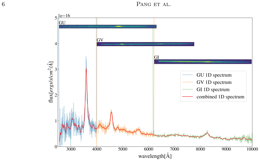
The load-bearing mechanism is the combination of three low-resolution grism spectra (GU, GV, and GI, covering 2550 to 10000 Å at $R \approx 200$) into a single continuum-normalized 548-point spectrum. That spectral vector feeds a convolutional neural network (RegNet) that outputs a four-way classification; the same combined spectrum is passed through a median-filter continuum subtraction, then emission-line peak detection and cross-correlation matching against a rest-frame line list to assign redshifts; QSOFITMORE then fits the pseudo-continuum, Fe II template, and multi-Gaussian line complexes. Because grism line profiles are convolved with the PSF, the FWHM outputs are calibrated against half of the simulated sample before applying virial mass estimators, and this calibration step is what allows 0.13 dex mass precision.
What would settle it
Run the identical pipeline on a mock field with realistic stellar density and overlapping grism spectra; if the quasar recovery fraction falls below the roughly 90% completeness assumed in the yield forecast, the headline figures do not transfer to the actual survey.
Extended reading notes
Core claim
On its own terms, the paper's discovery is a demonstrated end-to-end path from raw CSST grism images to science-ready quasar parameters. The pipeline simulates raw GU, GV, and GI grism exposures, extracts one-dimensional spectra, classifies sources with a RegNet convolutional network into low-redshift quasars, high-redshift quasars, galaxies, and stars, determines redshifts by matching detected emission-line peaks to a quasar line atlas, and estimates black hole masses and Eddington ratios with QSOFITMORE after calibrating emission-line FWHM values against the simulation input. The headline accuracy figures—99% classification, $\sigma_{\mathrm{NMAD}} = 0.002$ redshift scatter with 90% completeness, 0.13 dex mass scatter, 0.15 dex Eddington-ratio scatter, and a projected roughly 0.9 million new quasars—are what the survey would deliver if the simulation is faithful.
Load-bearing premise
The whole forecast rests on real CSST fields behaving like the sparse mock fields: crowding and spectral overlap are omitted from the simulation, and if contamination on the real sky cannot be controlled, the 99%, 90%, and 0.9-million numbers all degrade.
Editorial extensions
If this is right
- Roughly 0.9 million quasars not already in earlier survey catalogs would be newly identified by CSST grism spectroscopy alone.
- Ninety percent of classified quasars would carry redshifts precise to $\sigma_{\mathrm{NMAD}} \approx 0.002$, making the sample usable for clustering, luminosity-function, and large-scale-structure studies.
- Single-epoch black hole masses and Eddington ratios with about 0.13 and 0.15 dex scatter would give a very large statistical sample for accretion and black-hole-galaxy coevolution studies, before adding the systematic uncertainty of the virial calibration.
- Losing one of the three grism bands lowers classification accuracy to below 98%, and losing two degrades it further, so full GU+GV+GI coverage is what secures the headline performance.
- Metallicity diagnostics based on C III]/C IV and Fe II/Mg II are usable with roughly 0.18 dex scatter, while Si IV/C IV and weaker UV lines are not reliable enough for metallicity work.
Reading between the lines
- Editorial inference: the 0.9 million yield is best read as an upper anchor, because it inherits the assumed quasar luminosity function and subtracts previously cataloged objects; the realized count can shift with either input.
- Editorial inference: the key stress test the paper itself points to is contamination; since the mock fields are 30–45 times sparser than real star fields and overlapping grism spectra are not simulated, re-running the pipeline on crowded simulated fields would be more informative than further network tuning.
- Editorial inference: the 0.13 dex mass scatter is pipeline precision relative to simulated inputs, not total uncertainty on an individual real object, and systematic offsets from the single-epoch virial estimators would add on top.
- Editorial inference: artifacts at the grism band junctions create redshift-dependent quality variations, so scientific uses of the sample should carry redshift-dependent weights to avoid imprinting those artifacts on luminosity functions or metallicity evolution.
Editorial analysis
A structured set of objections, weighed in public.
Referee Report
Summary. This paper presents a pilot pipeline for identifying quasars and measuring their physical properties from mock Chinese Space Station Telescope (CSST) slitless spectroscopy. Using the CSST Cycle 6 simulation code, the authors generate sparse mock fields containing quasars, galaxies, and stars with r-band magnitudes 18<mr<22, extract one-dimensional grism spectra, classify objects with a RegNet convolutional neural network, measure redshifts by emission-line matching, and fit black hole masses and Eddington ratios with QSOFITMORE. They report 99% classification accuracy, 89.7% of successfully classified quasars with two or more emission-line detections and σ_NMAD=0.002, 0.13 dex scatter in black hole mass and 0.15 dex in Eddington ratio, and a forecast of roughly 0.9 million new quasars from the CSST wide survey.
Significance. The paper is a well-structured pilot study that uses publicly available simulation tools (CSST Cycle 6, SimQSO) and an open-source spectral fitting package (QSOFITMORE), and it provides quantitative robustness tests for missing grisms and source variability (Tables 4 and 5). These are genuine strengths. If the headline numbers hold, the CSST grism survey would deliver a large, homogeneously selected quasar sample with reliable redshifts and single-epoch black hole masses, complementing SDSS, DESI, and Gaia. However, the claimed performance is demonstrated only on sparse, uncontaminated mock fields with an ideal wavelength calibration; the realism gaps are acknowledged in Sections 6.3 and 6.4, yet the abstract and summary present the numbers without these caveats. The significance is therefore conditional on closing the class-prior and contamination gaps in the evaluation.
major comments (3)
- [§3, Table 4; §6.3; §7] The headline classification accuracy (99%, balanced accuracy 0.9921) is computed on a validation set with nearly balanced classes (1645 QSOs, 1255 galaxies, 1468 stars). On the real sky at 18<mr<22, quasars are a small minority, and the authors themselves state in §6.3 that 'only a few percent of the mis-classification of galaxies could lead to a disastrous drop in the accuracy of the QSO samples.' No precision or purity under realistic sky priors is reported, despite the fact that it can be estimated directly from the confusion matrix in Figure 6 combined with expected number counts. Because the forecast of ~0.9 million new quasars in §7 relies on the high QSO recall of this classifier, the class-prior issue is load-bearing for the central claim. I request a quantitative treatment: compute the expected QSO precision/purity after applying the confusion matrix to a realistic source mixture, or re-run the classifier on a mock field with realistic number densities, and present the resulting accuracy with an appropriate caveat.
- [§2.2, §6.4] The simulated fields are deliberately 30–45 times less dense than real star fields, and overlapping grism spectra are not modeled (§2.2). Section 6.4 discusses contamination qualitatively and adopts a literature-based ~10% contamination rate (Wen et al. 2024), but the impact of blending on the pipeline's classification, redshift measurement, and spectral fitting is never quantified. The CNN is trained exclusively on isolated 1D spectra, so the 99% classification accuracy, the ~90% two-line redshift completeness, and the 0.13/0.15 dex parameter scatters are upper limits. The 10% contamination rate is used only as a multiplicative completeness factor in the 0.9M forecast; it does not enter the measured performance metrics. I request an end-to-end test in which a fraction of mock spectra are blended with neighboring sources (or at least a simulation of the expected level of flux contamination) to assess how the pipeline degrades and how masking or forward-modeling would recover performance.
- [§5.1, Figure 10] The FWHM calibration relation is fitted on half the mock sample and applied to the full sample; the functional form is described only as a 'linear combination of the Gaussian width (σ), FWHM, and monochromatic luminosity,' and the fitted coefficients are not reported. This is a post-hoc correction calibrated on the same simulation, so the resulting 0.13 dex MBH scatter and 0.15 dex λEdd scatter measure internal reproducibility of the calibration rather than accuracy on independent data. I request that the authors publish the coefficients (or the exact fitting code), validate the relation with a proper held-out test (e.g., fitting on one redshift/magnitude subsample and testing on another), and, if possible, test on real quasar spectra degraded to CSST resolution. Without these steps, the physical-parameter uncertainties are not reproducible and do not yet account for the systematic effects of the low resolution and the unmodeled contamination.
minor comments (4)
- [§6.1, §1 (Abstract)] The abstract states σ_NMAD=0.002 without the caveat, given in §6.1, that this value assumes an ideal polynomial wavelength calibration; the paper estimates the actual scatter will be about 0.003. Please add the qualifier 'with ideal wavelength calibration' in the abstract and summary.
- [§5.2.1, Table 3] The text says the Si IV/C IV ratio has a scatter of 'up to 0.3 dex,' while Table 3 lists a scatter of 0.093; please clarify whether 0.3 dex is the maximum over specific redshift ranges and give both the global and worst-case values.
- [§2.2] The sentence 'The input wavelength for all mock data is standardized from 1500 Å to 12500 Å at a spectral resolution of 4000' is ambiguous; it should be clarified that 4000 is the resolution of the SED templates before convolution with the CSST grism line-spread function (R~200).
- [§7] The forecast of 'about 0.9 million new quasars' should be labeled as a projection that depends on the mock-based classification completeness and the assumed 10% contamination rate; please state the dependence and an approximate uncertainty on this number.
Circularity Check
Black-hole-mass and Eddington-ratio scatters are partly in-sample calibration residuals; classification and redshift claims are held-out mock validations.
-
fitted input called prediction
[Sec. 5.1 'Black Hole Mass and Eddington Ratio Estimation of QSOs'; Eqs. (9)-(11) and following text]
"Therefore, we fit the FWHM values using the linear combination of the Gaussian width (σ), FWHM, and monochromatic luminosity (L1350, L3000, L5100 corresponding to C IV, Mg II, Hβ) outputted by QSOFITMORE for half of the samples. Then we apply such linear relation to the entire sample set to get the calibrated FWHM value. Figure 10 compares the calibrated FWHM and the input spectra."
The calibration target is the input FWHM, so applying the fitted relation and then comparing the resulting FWHM, MBH, and λEdd with the input catalog measures, at least on the calibration half, the in-sample residual of a fit to the truth rather than an independent spectral-fitting prediction. FWHM enters MBH directly through Eqs. (9)-(11) and λEdd through MBH, so the advertised 0.13/0.15 dex scatters are partly forced by the calibration step. The paper does not state that the reported scatter is computed only on the held-out half, and the phrase 'entire sample set' suggests the calibration half is included.
full rationale
The main selection and redshift claims are not circular: the CNN is trained on a random 4:1 split of simulated spectra and evaluated on the held-out validation subset, and redshifts are obtained by matching detected peaks against the external Vanden Berk et al. line list, then compared with input redshifts. Those are standard simulation validations, and the 99% accuracy and σNMAD values have independent content within the mock. The one construction-level issue is in Sec. 5.1: the FWHM calibration is fitted to the input FWHM on half the sample, then applied to the entire sample, and the reported 0.13/0.15 dex scatter for MBH and λEdd is measured against the same input catalog. Because FWHM enters the virial estimators directly (Eqs. 9-11), that headline scatter is partly an in-sample residual of the calibration rather than an independent prediction. The paper's realism limitations (sparse mock fields, no contamination simulation, balanced class priors; Secs. 2.2, 6.3, 6.4) are external-validity concerns, not circularity, so they do not raise the score further.
Assumptions & free parameters
free parameters (4)
- FWHM calibration coefficients for C IV, Mg II, H beta =
not reported
- Emission-line matching weights and tolerances =
Table 1
- SNR thresholds for spectrum extraction =
SNR<5 per band; total SNR<9 rejected
- CNN architecture and training hyperparameters =
RegNet: 4 convolutional layers, 10 channels, kernel 5; FC layers 128/100/16; batch size 10; 200 epochs
assumptions (6)
- domain assumption The CSST Cycle 6 simulation code accurately reproduces CSST instrumental effects including PSF, distortion, PRNU, CTE, nonlinearity, and sensitivity curves.
- domain assumption SimQSO quasar spectra with eBOSS luminosity function statistics represent the real quasar population at z=0-5 in the CSST bands.
- domain assumption The sparse, uncontaminated simulated fields are sufficient to characterize survey performance; contamination is externally estimated at 5-10%.
- ad hoc to paper The linear FWHM calibration fitted on half of the mock sample is valid for the rest of the sample and for real data.
- domain assumption The single-epoch virial mass estimators and bolometric corrections from the literature apply to this sample.
- domain assumption The quasar luminosity functions of Paris et al. 2018 and Shen et al. 2020, plus overlap estimates from SDSS, Gaia, and DESI, yield 1.7 million total and 0.9 million new quasars.
Cite this review
Pith. "Pith review of A Pilot Study for the CSST Slitless Spectroscopic Quasar Survey Based on Mock Data." pith.science (2026). https://pith.science/paper/NQP33DLA
@misc{pith2026250112665,
  author       = {Pith},
  title        = {Pith review of: A Pilot Study for the CSST Slitless Spectroscopic Quasar Survey Based on Mock Data},
  year         = {2026},
  howpublished = {\url{https://pith.science/paper/NQP33DLA}},
  note         = {Machine review of arXiv:2501.12665}
}
abstract
The wide survey of the Chinese Space Station Telescope (CSST) will observe a large field of 17,500 $\text{deg}^2$. The GU, GV, and GI grism observations of CSST will cover a wavelength range from 2550 to 10000\r{A} at a resolution of $R\sim 200$ and a depth of about 22 AB magnitude for the continuum. In this paper, we present a pipeline to identify quasars and measure their physical properties with the CSST mock data. We simulate the raw images and extract the one-dimensional grism spectra for quasars, galaxies, and stars with the r-band magnitudes of $18<\text{m}_{\text{r}}<22$ using the CSST Cycle 6 simulation code. Using a convolution neural network, we separate quasars from stars and galaxies. We measure the redshifts by identifying the strong emission lines of quasars. We also fit the 1D slitless spectra with QSOFITMORE to estimate the black hole masses and Eddington ratios. Our results show that the CSST slitless spectroscopy can effectively separate quasars with redshifts $z=0-5$ from other types of objects with an accuracy of 99\%. Among those successfully classified quasars, 90\% of them could have precise redshift measurements with $\sigma_{\mathrm{NMAD}}=0.002$. The scatters of black hole masses and Eddington ratios from the spectral fittings are 0.13 and 0.15 dex, respectively. The metallicity diagnosis line ratios have a scatter of 0.1-0.2 dex. Our results show that the CSST slitless spectroscopy survey has the potential to discover about 0.9 million new quasars and provide important contributions to AGN science and cosmology.
Figures


Figures from the paper (10 more)


Reference graph
Works this paper leans on
-
[1]
Abdurro’uf, Accetta, K., Aerts, C., et al. 2022, ApJS, 259, 35, doi: 10.3847/1538-4365/ac4414 Allende Prieto, C., Koesterke, L., Hubeny, I., et al. 2018, A&A, 618, A25, doi: 10.1051/0004-6361/201732484
-
[2]
2023, JCAP, 2023, 043, doi: 10.1088/1475-7516/2023/11/043
Alonso, D., Fabbian, G., Storey-Fisher, K., et al. 2023, JCAP, 2023, 043, doi: 10.1088/1475-7516/2023/11/043
-
[3]
1993, ARA&A, 31, 473, doi: 10.1146/annurev.aa.31.090193.002353 Arrigoni Battaia, F., Hennawi, J
Antonucci, R. 1993, ARA&A, 31, 473, doi: 10.1146/annurev.aa.31.090193.002353 Arrigoni Battaia, F., Hennawi, J. F., Prochaska, J. X., &
arXiv 1993
-
[4]
2015, ApJ, 809, 163, doi: 10.1088/0004-637X/809/2/163
Cantalupo, S. 2015, ApJ, 809, 163, doi: 10.1088/0004-637X/809/2/163
-
[5]
Backhaus, B. E., Bridge, J. S., Trump, J. R., et al. 2023, ApJ, 943, 37, doi: 10.3847/1538-4357/aca668
-
[6]
Bentz, M. C., Peterson, B. M., Pogge, R. W., Vestergaard, M., & Onken, C. A. 2006, ApJ, 644, 133, doi: 10.1086/503537
doi:10.1086/503537 2006
-
[7]
Blanton, M. R., Bershady, M. A., Abolfathi, B., et al. 2017, AJ, 154, 28, doi: 10.3847/1538-3881/aa7567
-
[8]
Brammer, G. 2019, Grizli: Grism redshift and line analysis software, Astrophysics Source Code Library, record ascl:1905.001. http://ascl.net/1905.001 18 Pang et al
work page 2019
Show all 75 references
- [9]
- [10]
-
[11]
2023, Science China
Chen, Y., Fu, X., Liu, C., et al. 2023, Science China
2023
-
[12]
Physics, Mechanics, and Astronomy, 66, 119511, doi: 10.1007/s11433-023-2181-x
- [13]
-
[14]
2023, MNRAS, 522, 2019, doi: 10.1093/mnras/stad1007
Cristiani, S., Porru, M., Guarneri, F., et al. 2023, MNRAS, 522, 2019, doi: 10.1093/mnras/stad1007
2023 doi
-
[15]
S., Schlegel, D
Dawson, K. S., Schlegel, D. J., Ahn, C. P., et al. 2013, AJ, 145, 10, doi: 10.1088/0004-6256/145/1/10 De Rosa, G., Decarli, R., Walter, F., et al. 2011, ApJ, 739, 56, doi: 10.1088/0004-637X/739/2/56 DESI Collaboration, Adame, A. G., Aguilar, J., et al. 2023, arXiv e-prints, ar...
-
[16]
2016, ApJ, 825, 126, doi: 10.3847/0004-637X/825/2/126 Euclid Collaboration, Selwood, M., Fotopoulou, S., et al
Du, P., Lu, K.-X., Zhang, Z.-X., et al. 2016, ApJ, 825, 126, doi: 10.3847/0004-637X/825/2/126 Euclid Collaboration, Selwood, M., Fotopoulou, S., et al. 2024, arXiv e-prints, arXiv:2405.18126, doi: 10.48550/arXiv.2405.18126
2016 doi
-
[17]
Flesch, E. W. 2023, The Open Journal of Astrophysics, 6, 49, doi: 10.21105/astro.2308.01505
2023 arXiv
-
[18]
2021, QSOFITMORE: a python package for fitting UV- optical spectra of quasars, v1.1.0, Zenodo, doi: 10.5281/zenodo.5810042
Fu, Y. 2021, QSOFITMORE: a python package for fitting UV- optical spectra of quasars, v1.1.0, Zenodo, doi: 10.5281/zenodo.5810042
2021 doi
-
[19]
2022, ApJS, 261, 32, doi: 10.3847/1538-4365/ac7f3e
Fu, Y., Wu, X.-B., Jiang, L., et al. 2022, ApJS, 261, 32, doi: 10.3847/1538-4365/ac7f3e
2022 doi
-
[20]
2024, ApJS, 271, 54, doi: 10.3847/1538-4365/ad2ae6 Gaia Collaboration, Mignard, F., Klioner, S
Fu, Y., Wu, X.-B., Li, Y., et al. 2024, ApJS, 271, 54, doi: 10.3847/1538-4365/ad2ae6 Gaia Collaboration, Mignard, F., Klioner, S. A., et al. 2018, A&A, 616, A14, doi: 10.1051/0004-6361/201832916 Gaia Collaboration, Klioner, S. A., Lindegren, L., et al. 2022, A&A, 667, A148, do...
2024 doi
-
[21]
2018, PyQSOFit: Python code to fit the spectrum of quasars, Astrophysics Source Code Library, record ascl:1809.008
Guo, H., Shen, Y., & Wang, S. 2018, PyQSOFit: Python code to fit the spectrum of quasars, Astrophysics Source Code Library, record ascl:1809.008
2018
-
[22]
2002, ApJ, 564, 592, doi: 10.1086/324289
Baldwin, J. 2002, ApJ, 564, 592, doi: 10.1086/324289
2002 doi
-
[23]
2020, ARA&A, 58, 27, doi: 10.1146/annurev-astro-120419-014455
Inayoshi, K., Visbal, E., & Haiman, Z. 2020, ARA&A, 58, 27, doi: 10.1146/annurev-astro-120419-014455
2020 doi
-
[24]
2007, AJ, 134, 1150, doi: 10.1086/520811
Jiang, L., Fan, X., Vestergaard, M., et al. 2007, AJ, 134, 1150, doi: 10.1086/520811
2007 doi
-
[25]
2022, Nature Astronomy, 6, 850, doi: 10.1038/s41550-022-01708-w
Jiang, L., Ning, Y., Fan, X., et al. 2022, Nature Astronomy, 6, 850, doi: 10.1038/s41550-022-01708-w
2022 doi
- [26]
-
[27]
J., Matthee, J., et al
Kashino, D., Lilly, S. J., Matthee, J., et al. 2023, ApJ, 950, 66, doi: 10.3847/1538-4357/acc588
2023 doi
-
[28]
S., Netzer, H., et al
Kaspi, S., Smith, P. S., Netzer, H., et al. 2000, ApJ, 533, 631, doi: 10.1086/308704
2000 doi
-
[29]
Kormendy, J., & Ho, L. C. 2013, ARA&A, 51, 511, doi: 10.1146/annurev-astro-082708-101811 K¨ ummel, M., Walsh, J. R., Pirzkal, N., Kuntschner, H., &
2013 doi
-
[30]
2009, PASP, 121, 59, doi: 10.1086/596715
Pasquali, A. 2009, PASP, 121, 59, doi: 10.1086/596715
2009 doi
-
[31]
D., Walter, F., Fan, X., et al
Kurk, J. D., Walter, F., Fan, X., et al. 2007, ApJ, 669, 32, doi: 10.1086/521596
2007 doi
-
[32]
W., Prochaska, J
Lau, M. W., Prochaska, J. X., & Hennawi, J. F. 2016, ApJS, 226, 25, doi: 10.3847/0067-0049/226/2/25
2016 doi
-
[33]
W., Higley, A
Lyke, B. W., Higley, A. N., McLane, J. N., et al. 2020, ApJS, 250, 8, doi: 10.3847/1538-4365/aba623
2020 doi
-
[34]
2021, simqso: Simulated quasar spectra generator, Astrophysics Source Code Library, record ascl:2106.008
McGreer, I., Moustakas, J., & Schindler, J. 2021, simqso: Simulated quasar spectra generator, Astrophysics Source Code Library, record ascl:2106.008
2021
-
[35]
J., & Dunlop, J
McLure, R. J., & Dunlop, J. S. 2004, MNRAS, 352, 1390, doi: 10.1111/j.1365-2966.2004.08034.x
2004
-
[36]
G., Brammer, G
Momcheva, I. G., Brammer, G. B., van Dokkum, P. G., et al. 2016, ApJS, 225, 27, doi: 10.3847/0067-0049/225/2/27
2016 doi
-
[37]
J., Warren, S
Mortlock, D. J., Warren, S. J., Venemans, B. P., et al. 2011, Nature, 474, 616, doi: 10.1038/nature10159
2011 doi
-
[38]
2006, A&A, 447, 157, doi: 10.1051/0004-6361:20054024
Nagao, T., Marconi, A., & Maiolino, R. 2006, A&A, 447, 157, doi: 10.1051/0004-6361:20054024
2006 doi
-
[39]
2015, ARA&A, 53, 365, doi: 10.1146/annurev-astro-082214-122302
Netzer, H. 2015, ARA&A, 53, 365, doi: 10.1146/annurev-astro-082214-122302
2015 doi
-
[40]
1997a, NuPhA, 616, 79, doi: 10.1016/S0375-9474(97)00076-6
Nomoto, K., Hashimoto, M., Tsujimoto, T., et al. 1997a, NuPhA, 616, 79, doi: 10.1016/S0375-9474(97)00076-6
-
[41]
1997b, NuPhA, 621, 467, doi: 10.1016/S0375-9474(97)00291-1
Nomoto, K., Iwamoto, K., Nakasato, N., et al. 1997b, NuPhA, 621, 467, doi: 10.1016/S0375-9474(97)00291-1
-
[42]
2020, ApJ, 898, 105, doi: 10.3847/1538-4357/aba193 Pˆ aris, I., Petitjean, P., Aubourg,´E., et al
Onoue, M., Ba˜ nados, E., Mazzucchelli, C., et al. 2020, ApJ, 898, 105, doi: 10.3847/1538-4357/aba193 Pˆ aris, I., Petitjean, P., Aubourg,´E., et al. 2018, A&A, 613, A51, doi: 10.1051/0004-6361/201732445 Planck Collaboration, Abergel, A., Ade, P. A. R., et al. 2014, A&A, 571, ...
2020 doi
- [43]
-
[44]
Rees, M. J. 1986, MNRAS, 218, 25P, doi: 10.1093/mnras/218.1.25P
1986 doi
-
[45]
T., Lacy, M., Storrie-Lombardi, L
Richards, G. T., Lacy, M., Storrie-Lombardi, L. J., et al. 2006, ApJS, 166, 470, doi: 10.1086/506525 Pilot Study for the CSST Slitless Spectroscopic Quasar Survey 19
2006 doi
-
[46]
2017, in Society of Photo-Optical Instrumentation Engineers (SPIE) Conference Series, Vol
Rossin, C., Grange, R., Caillat, A., et al. 2017, in Society of Photo-Optical Instrumentation Engineers (SPIE) Conference Series, Vol. 10563, Society of Photo-Optical Instrumentation Engineers (SPIE) Conference Series, 105634W, doi: 10.1117/12.2304070
2017 doi
-
[47]
E., J., Casertano, S., & Pirzkal, N
Ryan, R. E., J., Casertano, S., & Pirzkal, N. 2018, PASP, 130, 034501, doi: 10.1088/1538-3873/aaa53e
2018 doi
-
[48]
2019, BAAS, 51, 413
Ryan, R., Malhotra, S., Pirzkal, N., et al. 2019, BAAS, 51, 413
2019
-
[49]
P., Ba˜ nados, E., et al
Schindler, J.-T., Farina, E. P., Ba˜ nados, E., et al. 2020, ApJ, 905, 51, doi: 10.3847/1538-4357/abc2d7
2020 doi
-
[50]
2020, ApJ, 899, 112, doi: 10.3847/1538-4357/aba8a1
Treister, E. 2020, ApJ, 899, 112, doi: 10.3847/1538-4357/aba8a1
2020 doi
-
[51]
F., Faucher-Gigu` ere, C.-A., et al
Shen, X., Hopkins, P. F., Faucher-Gigu` ere, C.-A., et al. 2020, MNRAS, 495, 3252, doi: 10.1093/mnras/staa1381
2020 doi
-
[52]
T., Strauss, M
Shen, Y., Richards, G. T., Strauss, M. A., et al. 2011, ApJS, 194, 45, doi: 10.1088/0067-0049/194/2/45
2011 doi
-
[53]
B., Horne, K., et al
Shen, Y., Hall, P. B., Horne, K., et al. 2019, ApJS, 241, 34, doi: 10.3847/1538-4365/ab074f
2019 doi
-
[54]
W., Rix, H.-W., et al
Storey-Fisher, K., Hogg, D. W., Rix, H.-W., et al. 2024, ApJ, 964, 69, doi: 10.3847/1538-4357/ad1328
2024 doi
-
[55]
R., Hall, P
Trump, J. R., Hall, P. B., Reichard, T. A., et al. 2006, ApJS, 165, 1, doi: 10.1086/503834
2006 doi
-
[56]
1995, MNRAS, 277, 945, doi: 10.1093/mnras/277.3.945
Tsujimoto, T., Nomoto, K., Yoshii, Y., et al. 1995, MNRAS, 277, 945, doi: 10.1093/mnras/277.3.945
1995 doi
-
[57]
M., & Padovani, P
Urry, C. M., & Padovani, P. 1995, PASP, 107, 803, doi: 10.1086/133630 Vanden Berk, D. E., Richards, G. T., Bauer, A., et al. 2001, AJ, 122, 549, doi: 10.1086/321167
1995 doi
-
[58]
Vestergaard, M., & Peterson, B. M. 2006, ApJ, 641, 689, doi: 10.1086/500572
2006 doi
-
[59]
2021, Nature Reviews Physics, 3, 732, doi: 10.1038/s42254-021-00364-9
Volonteri, M., Habouzit, M., & Colpi, M. 2021, Nature Reviews Physics, 3, 732, doi: 10.1038/s42254-021-00364-9
2021 doi
-
[60]
2021, ApJL, 907, L1, doi: 10.3847/2041-8213/abd8c6
Wang, F., Yang, J., Fan, X., et al. 2021, ApJL, 907, L1, doi: 10.3847/2041-8213/abd8c6
2021 doi
-
[61]
2012, ApJL, 751, L23, doi: 10.1088/2041-8205/751/2/L23
Wang, H., Zhou, H., Yuan, W., & Wang, T. 2012, ApJL, 751, L23, doi: 10.1088/2041-8205/751/2/L23
2012 doi
-
[62]
2009, ApJ, 707, 1334, doi: 10.1088/0004-637X/707/2/1334
Wang, J.-G., Dong, X.-B., Wang, T.-G., et al. 2009, ApJ, 707, 1334, doi: 10.1088/0004-637X/707/2/1334
2009 doi
-
[63]
2019, ApJ, 877, 116, doi: 10.3847/1538-4357/ab1c61
Wang, S., & Chen, X. 2019, ApJ, 877, 116, doi: 10.3847/1538-4357/ab1c61
2019 doi
-
[64]
Z., Han, Y., et al
Wen, R., Zheng, X. Z., Han, Y., et al. 2024, Monthly Notices of the Royal Astronomical Society, 528, 2770, doi: 10.1093/mnras/stae157
2024 doi
-
[65]
C., Curtis-Lake, E., Hainline, K
Williams, C. C., Curtis-Lake, E., Hainline, K. N., et al. 2018, ApJS, 236, 33, doi: 10.3847/1538-4365/aabcbb
2018 doi
-
[66]
B., Wang, R., Kong, M
Wu, X. B., Wang, R., Kong, M. Z., Liu, F. K., & Han, J. L. 2004, A&A, 424, 793, doi: 10.1051/0004-6361:20035845
2004 doi
-
[67]
2015, Nature, 518, 512, doi: 10.1038/nature14241
Wu, X.-B., Wang, F., Fan, X., et al. 2015, Nature, 518, 512, doi: 10.1038/nature14241
2015 doi
-
[68]
2020, ApJL, 897, L14, doi: 10.3847/2041-8213/ab9c26
Yang, J., Wang, F., Fan, X., et al. 2020, ApJL, 897, L14, doi: 10.3847/2041-8213/ab9c26
2020 doi
-
[69]
W., Connolly, A
Yip, C. W., Connolly, A. J., Szalay, A. S., et al. 2004a, AJ, 128, 585, doi: 10.1086/422429
-
[70]
W., Connolly, A
Yip, C. W., Connolly, A. J., Vanden Berk, D. E., et al. 2004b, AJ, 128, 2603, doi: 10.1086/425626
-
[71]
2011, Scientia Sinica Physica, Mechanica & Astronomica, 41, 1441, doi: 10.1360/132011-961
Zhan, H. 2011, Scientia Sinica Physica, Mechanica & Astronomica, 41, 1441, doi: 10.1360/132011-961
2011 doi
-
[72]
2018, in 42nd COSPAR Scientific Assembly, Vol
Zhan, H. 2018, in 42nd COSPAR Scientific Assembly, Vol. 42, E1.16–4–18
2018
-
[73]
2021, Chinese Science Bulletin, 66, 1290, doi: https://doi.org/10.1360/TB-2021-0016
Zhan, H. 2021, Chinese Science Bulletin, 66, 1290, doi: https://doi.org/10.1360/TB-2021-0016
2021 doi
-
[74]
2024, MNRAS, 529, 2777, doi: 10.1093/mnras/stae655
Zhang, H., Behroozi, P., Volonteri, M., et al. 2024, MNRAS, 529, 2777, doi: 10.1093/mnras/stae655
2024 doi
-
[75]
2012, ApJ, 758, 104, doi: 10.1088/0004-637X/758/2/104
Zuo, W., Wu, X.-B., Liu, Y.-Q., & Jiao, C.-L. 2012, ApJ, 758, 104, doi: 10.1088/0004-637X/758/2/104
2012 doi
Reviewed August 10, 2026 · model on record in the stance chip above.
Discussion (0). Continue with ORCID to comment.