REVIEW 3 major objections 5 minor 74 references
The typicality principle and its implications for statistics and data science
T0 review · 3 major / 5 minor · reviewed 2026-08-10 · deepseek-v4-flash
Pith's one-line read The paper claims that a theory is unwarranted when the data are sufficiently atypical under it, and that this 'typicality principle' can be operationalized as a goodness-of-fit-penalized likelihood giving consistent estimators and…
desk verdict Penalize by goodness-of-fit p-value: a genuinely new estimation idea, but the advertised resolution of the classic paradoxes outruns the proof. read the letter →
The pith
A machine-rendered reading of the paper's core claim, the machinery that carries it, and where it could break.
The reading
What carries the argument
The load-bearing object is the typicality measure in Eq (7), built from the regularized objective $\rho^{\mathrm{typ}}_\lambda(x,\theta) = \ell_x(\theta) - \lambda\, r^{\mathrm{typ}}_x(\theta)$, with $r^{\mathrm{typ}}_x(\theta)$ the negative log of a goodness-of-fit p-value. The centered statistic $R_\lambda(x,\theta)$ is the objective minus its fitted maximum, so the p-value-like tail probability of $R_\lambda$ under $P_\theta$ quantifies how unusual the observed data are for that parameter. Its calibration property (5), stated as a requirement in Section 5.1, is what turns the measure into valid tests and confidence sets via Propositions 1 and 2, and the Monte Carlo approximation in Eq (9) is what makes the contour computable in practice.
What would settle it
Simulate many datasets from a fixed member of the model, compute the typicality measure with the paper's Monte Carlo recipe at a moderate $M$, and check whether the empirical frequency of $\tau_X(\theta) \le \alpha$ exceeds $\alpha$; an excess for any $\theta$ would falsify the calibration claim, and repeated under-coverage of the confidence sets would falsify Proposition 2 as implemented.
Extended reading notes
Core claim
The paper's central claim is that typicality, not likelihood, should be the primitive notion in statistical inference. For each candidate parameter $\theta$, it defines the typicality measure $\tau_x(\theta) = P_\theta\{R_\lambda(X,\theta) \ge R_\lambda(x,\theta)\}$, the tail probability of the goodness-of-fit-penalized objective at the observed data; $\tau_x(\theta)$ near zero means the data are atypical under $\theta$. From this measure, the estimator $\check\theta(x)$ that maximizes $\tau_x(\theta)$ is a 'maximum typicality estimator,' and the set $\{\theta : \tau_x(\theta) \ge \alpha\}$ is claimed to be a nominal $100(1-\alpha)\%$ confidence set. The paper demonstrates the measure on the three problematic examples, where the ordinary maximum likelihood estimator is inconsistent, biased, or nonexistent, while the typicality-based contour concentrates near the true parameter and the confidence set contains the truth.
Load-bearing premise
The formal guarantees rely on the typicality measurement keeping its promised probability bounds: an 'unusual' result should occur at most $\alpha$ of the time under the model, and the paper states this as a requirement rather than proving it, while also assuming the Monte Carlo approximation is accurate enough to preserve those bounds.
Editorial extensions
If this is right
- Goodness-of-fit penalization can make point estimation consistent in the paired-means variance problem, where maximum likelihood systematically underestimates the variance by half.
- Confidence sets built from a calibrated typicality measure can exclude the naive maximum likelihood estimate while containing the true parameter, as in the mean-vector-length example.
- The typicality framework unifies point estimation, testing, and confidence sets without requiring a prior distribution, when the calibration property holds.
- The approach is deliberately free to violate the likelihood principle, gaining efficiency if the sampling model is trusted; a modified measure is available if the model is not trusted.
Reading between the lines
- Beyond the paper, the same goodness-of-fit penalty could be tested on over-parameterized machine-learning models, where the authors expect overfitting analogies to the mixture example.
- Beyond the paper, a principled choice of $\lambda$ could exploit the universal scale of p-values, unlike conventional penalty scales that depend on the model.
- Beyond the paper, the calibration of the Monte Carlo contour at finite $M$ deserves a dedicated simulation study, since the guarantee in Proposition 2 inherits any error in the approximation.
Editorial analysis
A structured set of objections, weighed in public.
Referee Report
Summary. The paper proposes a 'typicality principle'—roughly, that a hypothesis H about a parameter is unwarranted when the observed data x is sufficiently atypical under P_θ for θ ∈ H—and implements it through a penalized likelihood objective ρ_λ^{typ}(x,θ) = ℓ_x(θ) − λ r_x^{typ}(θ), where r_x^{typ}(θ) is the negative log of a goodness-of-fit p-value. The method is illustrated on Le Cam's normal mixture, the Neyman–Scott problem, and Stein's normal mean vector length, where maximum likelihood behaves badly. A more formal version of the principle defines a typicality measure τ_x(θ) as the p-value of a test based on the penalized relative likelihood R_λ(x,θ) in Eq. (8), and Propositions 1–2 claim frequentist Type I error control and nominal confidence sets. The paper also discusses connections to the likelihood principle, prediction principle, and inferential models.
Significance. The conceptual idea of using goodness-of-fit p-values as data-dependent penalties is interesting and connects to a broad literature on model checking, falsificationism, and possibility-theoretic inference. The formal framework in Section 5 is cleanly stated and, if the calibration property were established for the proposed construction, would provide a coherent route to confidence sets without a prior. The three examples are classic and important. However, the current manuscript's central point-estimation claims are supported only by selected simulations with a hand-tuned λ, and the paper itself defers the necessary consistency and tuning theory to future work. The formal uncertainty-quantification results are p-value tautologies conditional on an unproved calibration property for a data-dependent statistic, and the Monte Carlo implementation is not analyzed. The contribution is therefore a promising research program rather than a completed methodology, and the present version overclaims its results.
major comments (3)
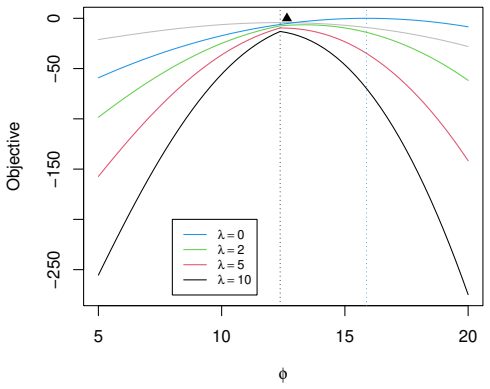
- [§4.2, §4.3, §6] The central point-estimation claim is not supported by a theorem or a tuning rule. In the Neyman–Scott problem, the objective in (1)–(2) has a log-likelihood term of order O(n) and a penalty term that is also O(n) through the large-deviation rate of the chi-square p-value, so consistency of σ̂²_λ for fixed λ can hold only above a problem-dependent threshold; the paper gives neither a threshold nor a data-driven selection rule. The evidence in Figure 5 is a single simulated dataset, and the sentence in §4.2 that the typicality principle 'resolves the Neyman–Scott paradox' is therefore an overclaim. The same issue appears in §4.3: the reported MSE comparison at λ=10 is one sentence with no replication details, and in the normal-mean-vector-length problem the penalty is bounded in n, so for fixed λ an O(1) bias can persist. The manuscript itself states in §6 that the finite- and large-sample efficiency properties are 'completely open' and that λ-selection is deferred; until these are provided, the examples demonstrate only that some λ values help in some simulations, not that the typicality principle repairs maximum likelihood failures as a general strategy.
- [§4.1] In the Le Cam mixture example, the text explicitly states that the Kolmogorov–Smirnov p-value does not depend on σ² at all, so the typicality penalty in (1)–(2) is constant in σ². The unboundedness of the likelihood as σ²→0 therefore remains unregularized, and the objective has no finite maximizer in σ²; the paper concedes 'challenges associated with optimizing over σ².' Consequently, the abstract's claim that the proposed regularization is effective in three nontrivial examples where maximum likelihood fails is not supported for this example: the method may correct the location parameter, but it leaves the variance component unidentified and the boundary problem unresolved. The paper should either narrow the claim or explain why the σ² component is outside the intended scope.
- [§5.1–5.2] Propositions 1 and 2 are immediate consequences of the calibration property (5) and are therefore p-value tautologies; the load-bearing requirement is that (5) actually holds for the specific data-dependent statistic R_λ in Eq. (8). The paper does not prove this: R_λ depends on the estimator ˇθ_x, no regularity or continuity conditions on its null distribution are stated, and the Monte Carlo approximation in Eq. (9) is used in Figure 7 without any analysis of its error. Thus the 'provably reliable uncertainty quantification' advertised in Section 5 is conditional on a property that is asserted for the proposed construction rather than verified. The paper should either prove calibration for R_λ under explicit conditions or explicitly state the exactness/approximation status of the guarantees and confidence sets.
minor comments (5)
- [§4.3, Eq. (3)] The quantity min{Q_φ²(‖x‖²), 1−Q_φ²(‖x‖²)} is not a valid two-tailed p-value; the usual two-tailed p-value is 2·min(Q, 1−Q). The constant factor 2 does not change the maximizer of the objective in (3), but the terminology is mathematically incorrect and should be corrected.
- [§1, §3, §6] There are minor typographical errors: 'Kullback–Leiber' should be 'Kullback–Leibler'; 'von Neumann and Morganstern' should be 'von Neumann and Morgenstern'; and 'An major challenge' should be 'A major challenge.'
- [§4.2, §4.3] The simulation evidence in Figures 5 and 6 lacks replication details: the number of Monte Carlo replications, standard errors, and a table of MSE values are not reported. The text should provide these to support the claimed efficiency comparisons.
- [§5.4] The statement that the contours for different λ are 'all peaked at effectively the same point' is based on a single simulated data set; either provide repeated-sampling evidence or soften the wording to a data-dependent observation.
- [References] Several key methodological ingredients are drawn from the authors' previous work (e.g., Martin and Liu 2015a, Martin 2024, Jiang and Liu 2025); citing independent treatments of p-value-based regularization or goodness-of-fit penalties would help the reader assess the novelty and situate the proposal in the broader literature.
Circularity Check
Formal UQ propositions are p-value tautologies; regularized-estimator claims rest on hand-tuned λ and are under-derived, but not circular.
-
self definitional
[Section 5.1, Propositions 1–2; Section 5.2, Eqs (7)–(8)]
"τx(θ) = Pθ{Rλ(X, θ) ≥ Rλ(x, θ)} ... Proposition 2. The set Cα(x) = {θ ∈ T : τx(θ) ≥ α} ... is a nominal 100(1 − α)% confidence set for Θ in the sense that sup_{θ∈T} Pθ{Cα(X) ̸∋ θ} ≤ α"
By (7), τ_x(θ) is, by definition, a P_θ-tail probability. The event that the Proposition 2 confidence set fails to cover θ is exactly {τ_X(θ) ≤ α}, so the asserted coverage bound sup_θ P_θ{τ_X(θ) ≤ α} ≤ α is precisely the calibration property (5) that Section 5.1 imposes as a requirement ('it makes sense to require'). Thus the nominal confidence-set guarantee is not derived from a proved property of the specific R_λ in (8); it is a restatement of the assumed calibration, and the Monte Carlo approximation (9) can only introduce additional error. The formal UQ claim is true by construction conditional on an exact calibrated p-value.
full rationale
The paper's central methodological contribution—typicality-based regularization in Eq (1)–(2) and its three examples—is not circular: the penalty is a goodness-of-fit p-value, the estimator is a penalized MLE, and the favorable behavior is demonstrated by simulation with explicitly hand-picked λ. The absence of a consistency theorem or data-driven λ rule is a scientific gap, not a circularity. The numerous citations to Martin, Liu, Cella, and Jiang are self-citations, but they are used for context, extensions, or implementation details (e.g., uniform-in-H validity, likelihood-principle modification, Monte Carlo methods), not as the load-bearing justification for the main claims; none of the examples or the regularization construction depends on an unverified uniqueness theorem from the authors. The one genuine reduction-by-construction is in Section 5: Proposition 1 and Proposition 2 simply restate the calibration property (5) after τ_x(θ) has been defined in (7) as a P_θ-tail probability. For Proposition 2, the coverage event C_α(X)∋θ is exactly τ_X(θ)≥α, so the asserted coverage bound is literally P_θ{τ_X(θ)≤α}≤α, which was imposed as a requirement rather than proved for the specific R_λ. The Monte Carlo approximation (9) is an additional numerical device that can only add error. Because the paper is explicit that (5) is a requirement, this is a transparent tautology rather than a hidden fit, but it does mean the 'provably reliable' UQ claims are true by definition conditional on an exact calibrated p-value. Overall score 4: partial definitional circularity in the formal UQ propositions, while the principal regularization/example content remains independent and non-circular.
Assumptions & free parameters
free parameters (1)
- lambda (tuning parameter) =
hand-picked: 0,1,2,5 in Neyman-Scott; 10 in Stein; varying in Le Cam
assumptions (4)
- domain assumption There exists a true parameter Theta and the posited model is correctly specified.
- domain assumption Prior information about Theta is vacuous.
- ad hoc to paper The typicality measure tau_x(theta) satisfies the calibration property in Eq (5).
- domain assumption For the Kolmogorov-Smirnov penalty, the data are iid and F_theta is continuous.
Cite this review
Pith. "Pith review of The typicality principle and its implications for statistics and data science." pith.science (2026). https://pith.science/paper/L2XPPIQE
@misc{pith2026250114860,
  author       = {Pith},
  title        = {Pith review of: The typicality principle and its implications for statistics and data science},
  year         = {2026},
  howpublished = {\url{https://pith.science/paper/L2XPPIQE}},
  note         = {Machine review of arXiv:2501.14860}
}
read the original abstract
A central focus of data science is the transformation of empirical evidence into knowledge. As such, the key insights and scientific attitudes of deep thinkers like Fisher, Popper, and Tukey are expected to inspire exciting new advances in machine learning and artificial intelligence in years to come. Along these lines, the present paper advances a novel {\em typicality principle} which states, roughly, that if the observed data is sufficiently ``atypical'' in a certain sense relative to a posited theory, then that theory is unwarranted. This emphasis on typicality brings familiar but often overlooked background notions like model-checking to the inferential foreground. One instantiation of the typicality principle is in the context of parameter estimation, where we propose a new typicality-based regularization strategy that leans heavily on goodness-of-fit testing. The effectiveness of this new regularization strategy is illustrated in three non-trivial examples where ordinary maximum likelihood estimation fails miserably. We also demonstrate how the typicality principle fits within a bigger picture of reliable and efficient uncertainty quantification.
Figures


Figures from the paper (4 more)



Reference graph
Works this paper leans on
-
[1]
Aldrich, J. (1997). R. A . F isher and the making of maximum likelihood 1912--1922. Statist. Sci. , 12(3):162--176
work page 1997
-
[2]
Basu, D. (1975). Statistical information and likelihood. Sankhy\= a Ser. A , 37(1):1--71. Discussion and correspondance between Barnard and Basu
1975
-
[3]
Basu, D. (1977). On the elimination of nuisance parameters. J. Amer. Statist. Assoc. , 72(358):355--366
1977
-
[4]
Berger, J. O., Bernardo, J. M., and Sun, D. (2009). The formal definition of reference priors. Ann. Statist. , 37(2):905--938
work page 2009
-
[5]
Berger, J. O. and Wolpert, R. L. (1984). The L ikelihood P rinciple . Institute of Mathematical Statistics Lecture Notes---Monograph Series, 6. Institute of Mathematical Statistics, Hayward, CA
work page 1984
-
[6]
Birnbaum, A. (1962). On the foundations of statistical inference. J. Amer. Statist. Assoc. , 57:269--326
1962
-
[7]
Carnap, R. (1962). Logical F oundations of P robability . Second edition. The University of Chicago Press, Chicago, Ill
work page 1962
-
[8]
and Martin, R
Cella, L. and Martin, R. (2023). Possibility-theoretic statistical inference offers performance and probativeness assurances. Internat. J. Approx. Reason. , 163:109060
2023
Show all 74 references
-
[9]
Datta, G. S. and Ghosh, J. K. (1995). On priors providing frequentist validity for B ayesian inference. Biometrika , 82(1):37--45
1995
-
[10]
Dempster, A. P. (1966). New methods for reasoning towards posterior distributions based on sample data. Ann. Math. Statist. , 37:355--374
1966
-
[11]
Dempster, A. P. (2002). John W . T ukey as ``philosopher''. Ann. Statist. , 30(6):1619--1628. In memory of John W. Tukey
2002
-
[12]
Dempster, A. P. (2008). The D empster-- S hafer calculus for statisticians. Internat. J. Approx. Reason. , 48(2):365--377
2008
-
[13]
Dubois, D., Foulloy, L., Mauris, G., and Prade, H. (2004). Probability-possibility transformations, triangular fuzzy sets, and probabilistic inequalities. Reliab. Comput. , 10(4):273--297
2004
-
[14]
and Prade, H
Dubois, D. and Prade, H. (1988). Possibility T heory . Plenum Press, New York
1988
-
[15]
Durbin, J. (1970). On B irnbaum's theorem on the relation between sufficiency, conditionality and likelihood. J. Amer. Statist. Assoc. , 65(329):395--398
1970
-
[16]
Edwards, A. W. F. (1992). Likelihood . Johns Hopkins University Press, Baltimore, MD, expanded edition. Revised reprint of the 1972 original
1992
-
[17]
Eschker, S. J. and Liu, C. (2024). Towards strong ai: Transformational beliefs and scientific creativity. arXiv preprint arXiv:2412.19938
2024 arXiv
-
[18]
Evans, M. (2013). What does the proof of B irnbaum's theorem prove? Electron. J. Stat. , 7:2645--2655
2013
-
[19]
Fisher, R. A. (1922). On the mathematical foundations of theoretical statistics. Philos. Trans. Roy. Soc. London Ser. A , 222:309--368
1922
-
[20]
Fisher, R. A. (1925). Theory of statistical estimation. Proc. Cambridge Philos. Soc. , 22:200--225
1925
-
[21]
Fisher, R. A. (1933). The concepts of inverse probability and fiducial probability referring to unknown parameters. Proc. R. Soc. Lond. A. , 139:343--348
1933
-
[22]
Fisher, R. A. (1935a). The fiducial argument in statistical inference. Ann. Eugenics , 6:391--398
1935
-
[23]
Fisher, R. A. (1935b). The logic of inductive inference. J. Roy. Statist. Soc. , 98:39--82
1935
-
[24]
Fraser, D. A. S. (1968). The S tructure of I nference . John Wiley & Sons Inc., New York
1968
-
[25]
Fraser, D. A. S., Reid, N., and Lin, W. (2018). When should modes of inference disagree? S ome simple but challenging examples. Ann. Appl. Stat. , 12(2):750--770
2018
-
[26]
Hacking, I. (1976). Logic of S tatistical I nference . Cambridge University Press, Cambridge-New York-Melbourne
1976
-
[27]
Hannig, J., Iyer, H., Lai, R. C. S., and Lee, T. C. M. (2016). Generalized fiducial inference: a review and new results. J. Amer. Statist. Assoc. , 111(515):1346--1361
2016
-
[28]
Hinton, G., Vinyals, O., and Dean, J. (2015). Distilling the knowledge in a neural network. arXiv preprint arXiv:1503.02531
2015 arXiv
-
[29]
Hose, D. (2022). Possibilistic R easoning with I mprecise P robabilities: S tatistical I nference and D ynamic F iltering . PhD thesis, University of Stuttgart. https://dominikhose.github.io/dissertation/diss_dhose.pdf
2022
-
[30]
Jaynes, E. T. (2003). Probability T heory . Cambridge University Press, Cambridge
2003
-
[31]
Jeffreys, H. (1946). An invariant form for the prior probability in estimation problems. Proc. Roy. Soc. London Ser. A , 186:453--461
1946
-
[32]
Jeffreys, H. (1998). Theory of P robability . Oxford Classic Texts in the Physical Sciences. The Clarendon Press, Oxford University Press, New York. Reprint of the 1983 edition
1998
-
[33]
and Liu, C
Jiang, Y. and Liu, C. (2025). Estimation of over-parameterized models from an auto-modeling perspective. To appear in J. Amer. Statist. Assoc., DOI: 10.1080/01621459.2025.2455192, arXiv:2206.01824
2025
-
[34]
Jiang, Y., Liu, C., and Zhang, H. (2023). Finite sample valid inference via calibrated bootstrap. arXiv:2408.16763
2023 arXiv
-
[35]
Le Cam, L. (1986). Asymptotic M ethods in S tatistical D ecision T heory . Springer Series in Statistics. Springer-Verlag, New York
1986
-
[36]
Le Cam, L. (1990). Maximum likelihood: A n introduction. Int. Stat. Rev. , 58(2):153--171
1990
-
[37]
Lehmann, E. (1983). Theory of Point Estimation . Wadsworth & Brooks/Cole Advanced Books & Software, Pacific Grove, California
1983
-
[38]
Liu, C. (2023). Reweighted and circularised A nderson- D arling tests of goodness-of-fit. J. Nonparametr. Stat. , 35(4):869--904
2023
-
[39]
Martin, R. (2015). Plausibility functions and exact frequentist inference. J. Amer. Statist. Assoc. , 110(512):1552--1561
2015
-
[40]
Martin, R. (2018). On an inferential model construction using generalized associations. J. Statist. Plann. Inference , 195:105--115
2018
-
[41]
Martin, R. (2021a). An imprecise-probabilistic characterization of frequentist statistical inference. arXiv:2112.10904
2021 arXiv
-
[42]
Martin, R. (2021b). Inferential models and the decision-theoretic implications of the validity property. arXiv:2112.13247
2021 arXiv
-
[43]
Martin, R. (2022a). Valid and efficient imprecise-probabilistic inference with partial priors, I . F irst results. arXiv:2203.06703
2022 arXiv
-
[44]
Martin, R. (2022b). Valid and efficient imprecise-probabilistic inference with partial priors, II . G eneral framework. arXiv:2211.14567
2022 arXiv
-
[45]
Martin, R. (2023a). Fiducial inference viewed through a possibility-theoretic inferential model lens. In Miranda, E., Montes, I., Quaeghebeur, E., and Vantaggi, B., editors, Proceedings of the Thirteenth International Symposium on Imprecise Probability: Theories and Applicatio...
2023
-
[46]
Martin, R. (2023b). Valid and efficient imprecise-probabilistic inference with partial priors, III . M arginalization. arXiv:2309.13454
2023 arXiv
-
[47]
Martin, R. (2024). A possibility-theoretic solution to B asu's B ayesian--frequentist via media. Sankhya A , 86:43--70
2024
-
[48]
Martin, R. (2025). A new M onte C arlo method for valid prior-free possibilistic statistical inference. arXiv:2501.10585
2025 arXiv
-
[49]
and Liu, C
Martin, R. and Liu, C. (2013). Inferential models: a framework for prior-free posterior probabilistic inference. J. Amer. Statist. Assoc. , 108(501):301--313
2013
-
[50]
and Liu, C
Martin, R. and Liu, C. (2014). Discussion: Foundations of statistical inference, revisited. Statist. Sci. , 29:247--251
2014
-
[51]
and Liu, C
Martin, R. and Liu, C. (2015a). Inferential M odels , volume 147 of Monographs on Statistics and Applied Probability . CRC Press, Boca Raton, FL
2015
-
[52]
and Liu, C
Martin, R. and Liu, C. (2015b). Marginal inferential models: prior-free probabilistic inference on interest parameters. J. Amer. Statist. Assoc. , 110(512):1621--1631
2015
-
[53]
Martin, R., Mess, R., and Walker, S. G. (2017). Empirical B ayes posterior concentration in sparse high-dimensional linear models. Bernoulli , 23(3):1822--1847
2017
-
[54]
and Walker, S
Martin, R. and Walker, S. G. (2019). Data-dependent priors and their posterior concentration rates. Electron. J. Stat. , 13(2):3049--3081
2019
-
[55]
Mayo, D. (2014). On the B irnbaum argument for the strong likelihood principle. Statist. Sci. , 29(2):227--239
2014
-
[56]
Molchanov, I. (2005). Theory of R andom S ets . Probability and Its Applications (New York). Springer-Verlag London Ltd., London
2005
-
[57]
and Scott, E
Neyman, J. and Scott, E. L. (1948). Consistent estimates based on partially consistent observations. Econometrica , 16:1--32
1948
-
[58]
Pardo, L. (2018). Statistical Inference Based on Divergence Measures . Chapman and Hall/CRC
2018
-
[59]
Popper, K. R. (1959). The L ogic of S cientific D iscovery . Hutchinson and Co., Ltd., London
1959
-
[60]
Shafer, G. (1976). A M athematical T heory of E vidence . Princeton University Press, Princeton, N.J
1976
-
[61]
Shafer, G. (1982). Belief functions and parametric models. J. Roy. Statist. Soc. Ser. B , 44(3):322--352. With discussion
1982
-
[62]
Stein, C. (1956). Inadmissibility of the usual estimator for the mean of a multivariate normal distribution. In Proceedings of the T hird B erkeley S ymposium on M athematical S tatistics and P robability, 1954--1955, vol. I , pages 197--206, Berkeley and Los Angeles. Universi...
1956
-
[63]
Stein, C. (1959). An example of wide discrepancy between fiducial and confidence intervals. Ann. Math. Statist. , 30:877--880
1959
-
[64]
Stigler, S. M. (2007). The epic story of maximum likelihood. Statist. Sci. , 22(4):598--620
2007
-
[65]
Tibshirani, R. (1989). Noninformative priors for one parameter of many. Biometrika , 76(3):604--608
1989
-
[66]
Troffaes, M. C. M. and de Cooman, G. (2014). Lower P revisions . Wiley Series in Probability and Statistics. John Wiley & Sons, Ltd., Chichester
2014
-
[67]
Tukey, J. W. (1962). The future of data analysis. In Breakthroughs in Statistics: Methodology and Distribution , pages 408--452. Springer
1962
-
[68]
Tukey, J. W. (1977). Exploratory D ata A nalysis . Pearson
1977
-
[69]
Tukey, J. W. (1986). The C ollected W orks of J ohn W . T ukey. V ol. III . The Wadsworth & Brooks/Cole Statistics/Probability Series. Wadsworth & Brooks/Cole Advanced Books & Software, Monterey, CA. Philosophy and principles of data analysis: 1949--1964, Edited and with comme...
1986
-
[70]
van der Vaart, A. (2002). The statistical work of L ucien L e C am. Ann. Statist. , 30(3):631--682. Dedicated to the memory of Lucien Le Cam
2002
-
[71]
N., Kaiser, L
Vaswani, A., Shazeer, N., Parmar, N., Uszkoreit, J., Jones, L., Gomez, A. N., Kaiser, L. u., and Polosukhin, I. (2017). Attention is all you need. In Guyon, I., Luxburg, U. V., Bengio, S., Wallach, H., Fergus, R., Vishwanathan, S., and Garnett, R., editors, Advances in Neural ...
2017
-
[72]
Walley, P. (1991). Statistical R easoning with I mprecise P robabilities , volume 42 of Monographs on Statistics and Applied Probability . Chapman & Hall Ltd., London
1991
-
[73]
and Singh, K
Xie, M. and Singh, K. (2013). Confidence distribution, the frequentist distribution estimator of a parameter: a review. Int. Stat. Rev. , 81(1):3--39
2013
-
[74]
Zabell, S. L. (1992). R. A . F isher and the fiducial argument. Statist. Sci. , 7(3):369--387
1992
Reviewed August 10, 2026 · model on record in the stance chip above.
Discussion (0). Continue with ORCID to comment.