REVIEW 3 major objections 6 minor 60 references
Disentangling Safe and Unsafe Corruptions via Anisotropy and Locality
T0 review · 3 major / 6 minor · reviewed 2026-08-10 · deepseek-v4-flash
Pith's one-line read Projected Displacement (PD) threat measures a perturbation by how well it aligns with directions that change the true label, allowing safe corruptions like blur and compression to be distinguished from unsafe ones of equal ℓp size.
desk verdict Projected Displacement is a genuinely new, practical threat model with a clean exact theory, but its central empirical claim rests on a calibrated heuristic and one evaluation table contains impossible numbers. read the letter →
The pith
A machine-rendered reading of the paper's core claim, the machinery that carries it, and where it could break.
The reading
What carries the argument
The central object is the set of observed unsafe directions U(x): unit vectors from an input x toward k-center representatives of each other class's training data, together with the normalization gβ(x,u)=β||x̃−x||2, β=1/2. The PD threat is the maximum over these directions of the positive projection ⟨δ,u⟩ divided by that normalization. This turns each ε-sublevel set into an intersection of halfspaces {δ : ⟨δ,u⟩ ≤ ε gβ(x,u)}, which is convex and admits fast projection, and it makes the threat grow linearly along any fixed direction.
What would settle it
Take an ImageNet image x and a k-center representative x̃ of another class, and move from x toward x̃ by distance t·||x̃−x||2 with t just above the true distance to the decision boundary. If t < β (with β=1/2), then d_PD(x, ·) < 1 along that direction while x + t·unit has a different true label, so the ε=1 sublevel set admits an unsafe perturbation; searching for such low-margin pairs in the training data would settle the calibration assumption.
Extended reading notes
Core claim
The paper's central claim is that the PD threat function distinguishes safe from unsafe perturbations of equal ℓp norm: noise, blur, and compression receive small PD threat, while perturbations that actually change the true class receive large PD threat. The exact version, PD⋆, is defined from the true class partition and satisfies a consistency theorem: the true labeling function is 1-robust at every input under PD⋆, meaning the permissible set never contains an unsafe perturbation. The empirical version approximates unsafe directions using representative training points of other classes and a heuristic normalization gβ(x,u)=β||x̃−x||2 with β=1/2. On ImageNet-1k, this empirical PD threat matches the DreamSim perceptual baseline in separating safe and unsafe corruptions, while requiring no pretraining or human similarity judgments.
Load-bearing premise
The load-bearing premise is the empirical calibration that the true decision boundary along each unsafe direction lies at about half the distance to the nearest representative training point of another class; if the boundary is much closer, a label-changing perturbation could still have PD threat below 1.
Editorial extensions
If this is right
- Under PD, robust accuracy on ImageNet-1k improves uniformly for benchmark classifiers compared with ℓ∞, and some models rank higher, meaning ℓ∞ leaderboards may misorder models.
- Because PD sublevel sets are convex and projections are available, existing white-box attacks can be adapted to evaluate robustness under PD directly.
- Segmentation masks and class hierarchies can be plugged into the threat without losing convexity, allowing robustness to be evaluated with task-specific sensitivities.
- PD can be computed for any classification task from training data alone, whereas perceptual threat models need pretraining and human similarity judgments.
Reading between the lines
- Editorial: because β is a single global constant, PD's ordering is likely fragile for low-margin inputs; calibrating β per input or per class from validation data would be a direct test of that fragility.
- Editorial: the exact PD threat is a data-driven estimator of distance to the true decision boundary; the paper leaves open sample-complexity guarantees on how the k-center selection and β affect the ε=1 sublevel set.
- Editorial: PD's convex, linear sublevel sets make it a natural regularizer for training; one could penalize alignment with unsafe directions directly, something the paper does not explore.
Editorial analysis
A structured set of objections, weighed in public.
Referee Report
Summary. The paper introduces Projected Displacement (PD), a threat function for classification robustness that is local and anisotropic. The exact version d*_PD (Definition 5) assumes knowledge of the true labeling function h*: unsafe directions U*(x) are those along which moving inside the input domain changes the true label, and g*(x,u) is the distance from x to the boundary of the true class along u. The threat of a perturbation is the maximal positive projection onto any unsafe direction, normalized by g*. Theorem 1 shows that h* is 1-robust under d*_PD. Since h* is unknown, the practical version (Definition 7) approximates U* by directions to k representative training points of each other class and replaces g* by beta times the distance to the representative point, with default (k,beta) = (50,1/2). The sublevel sets are convex polytopes, enabling projection-based attacks. Experiments on ImageNet compare PD with l_infty/l_2 and DreamSim on safe common corruptions vs. unsafe cross-class differences, and Section 6 evaluates RobustBench models under an intersection threat model. Extensions PD-S and PD-W incorporate segmentation masks and WordNet class distances.
Significance. If the practical PD threat reliably separated safe and unsafe perturbations, it would be a genuinely useful task-aware alternative to l_p threat models and to pretrained perceptual metrics, with convex sublevel sets, linear growth, and no need for foundation-model training. The exact formulation is clean, and the proof of Theorem 1 is sound. The paper also advertises a code repository, which is a strength for reproducibility. However, the central separation claim currently rests on a heuristic normalization and on average statistics, so the practical significance is not yet established. The contribution is substantial enough to warrant a revision rather than rejection.
major comments (3)
- [Section 3.2, Definition 7, and Theorem 1] The load-bearing claim that S(x,dPD,1) excludes unsafe perturbations is not a consequence of the theory. Theorem 1 is proved for d*_PD, whose normalization g*(x,u) is the true distance along u to the boundary of X_{h*(x)}. In the practical threat, g_beta(x,u) = beta ||x_tilde - x||_2 replaces g* by a fraction of the distance to a representative training point of another class. These two quantities are unrelated in general: for an unsafe direction u with representative x_tilde, if g*(x,u) = c ||x_tilde - x||_2 for some c < 1/2, then the label-changing perturbation delta = t u at t = c ||x_tilde - x||_2 satisfies dPD(x,delta) = 2c < 1, so it belongs to S(x,dPD,1). The kmin condition in Section 3.2 enforces dPD > 1 only on the training pairs used for calibration; it gives no control on validation inputs or on directions not represented in U_k(x). To support the abstract's claim, the paper needs either a transferable guarantee for dPD or a per-instance empirical verification that dPD > 1 holds for unsafe perturbations with high coverage.
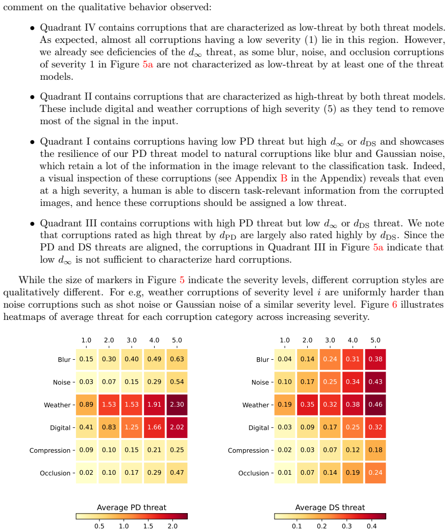
- [Section 4.2, Figure 5, and Tables 4-5] The empirical evidence is aggregate. Figure 5 reports per-corruption-style averages of dPD over 5,000 images, and Table 4 reports a single example. Averages can hide large fractions of unsafe perturbations with dPD <= 1 and safe corruptions with dPD > 1; they therefore cannot establish the "for any input" claim in the abstract. In addition, the threshold epsilon = 1 is chosen to be about half of the average unsafe threat, and the hyper-parameters k and beta are calibrated on the same type of unsafe/safe labels used in the evaluation, so the observed separation is partly by construction. Please report per-instance or quantile statistics, for example the fraction of unsafe pairs with dPD(x,x_tilde - x) <= epsilon as a function of epsilon, and verify at the image level that the "safe" corruptions actually preserve the true label for the evaluated inputs.
- [Section 6, Table 3] The reported robust accuracies under (d_infty cap dPD, epsilon) do not come from an adaptive attack for the intersection threat model. The text says that AutoAttack is run for d_infty and the resulting perturbation is then projected onto S(x,dPD,epsilon). Projection after the attack can only move the perturbation to a point that is not adversarial, so the numbers are optimistic upper bounds rather than adversarial robustness evaluations. An evaluation under the intersection requires an attack that projects onto S(x,d_infty,epsilon) cap S(x,dPD,epsilon) at each iteration, or a certified method; alternatively, Table 3 should be presented as a heuristic attack. This matters because the uniform improvement over d_infty in Table 3 may be an artifact of the weaker post-hoc attack.
minor comments (6)
- [Definition 5] The normalization function is denoted g*(u,x) in the display of Eq. (1) but g*(x,u) in the surrounding text; please use one consistent convention.
- [Section 3.2, 'Quality of Approximation'] The inequality dPD,k,1 <= d*_PD,k,beta refers to an undefined quantity d*_PD,k,beta; the comparison should be stated against d*_PD, using the fact that g*(x,u) <= ||x_tilde - x||_2.
- [Section 3.2, definition of kmin] Please specify that (x_tilde,c) runs over training points with c != y; otherwise same-label pairs are included in the minimization.
- [Theorem 1] Since delta = 0 is in every sublevel set, a classifier that is not 1-robust at x is already wrong at x; the second clause as stated is close to a tautology, and the more informative content is in the proof's Case 2.
- [Figure 3 captions] The captions write S(d*_PD,x,1) whereas the text defines S(x,d,epsilon); please align the notation.
- [Appendix Tables 4-5] The red/orange color legend is explained in the text but not in the table captions; please repeat the legend in each caption.
Circularity Check
The ε=1 exclusion of unsafe perturbations is calibrated into the practical PD model via kmin and β=1/2, and the empirical threshold is chosen as half the average unsafe threat, making the central disentangling claim partially circular.
-
fitted input called prediction
[Section 3.2 (Quality of Approximation, kmin definition and β=1/2 heuristic)]
"Given training data S, we first recommend finding the minimum k such that PD threat dPD,k,β rates unsafe corruptions on training data as a sufficiently large threat, kmin := min_{k∈[1, |S|/C]} s.t. min_{(x,y), (\tilde{x},c)∈S} dPD,k,β(x, \tilde{x} − x) > 1 ... Hence, in practice, we make a heuristic choice of β = 1/2 to compute the approximate normalization."
The ε=1 exclusion property is not a consequence of Theorem 1 for the practical threat: it is imposed by choosing kmin so that every unsafe training pair (x, x̃) has dPD,k,β(x, x̃−x) > 1, and by setting β=1/2 so the full displacement to an other-class training point has threat 2. The exact normalization g*(x,u) is the true distance to the decision boundary along u; the heuristic gβ=0.5·||x̃−x|| can overestimate it by an arbitrary factor. If the true boundary is closer than half the representative distance, a perturbation t·u with dPD<1 already changes the true label, so the permissible set S(x,dPD,1) is not guaranteed to exclude unsafe perturbations.
-
fitted input called prediction
[Section 4.2 (Disentangling Safe and Unsafe Corruption, threshold selection for Figure 5)]
"These thresholds were chosen to approximately be half of the average threat of unsafe perturbations that alter the true label. Admittedly, this binary threshold is coarse, and the Appendix contains fine-grained qualitative examples of corruptions of varying threat."
The claimed disentangling is evaluated by drawing a horizontal line at ε=1 for dPD and noting that the 'Unsafe' point (average dPD over validation pairs of different classes) lies above it while most common corruptions lie below. But the threshold ε=1 was explicitly chosen to be approximately half the average unsafe threat, so the separation of the average unsafe point from low-threat safe points is a restatement of the threshold calibration. The paper reports only avg(dPD,ω) and avg(dPD,unsafe), i.e., averages over 5000 images, not per-instance counts or quantiles; averages can be dominated by a few large values, and a threshold placed at half an average cannot certify that the ε=1 sublevel set excludes unsafe perturbations for individual inputs.
full rationale
The exact PD* construction (Definitions 4–5 and Theorem 1) is self-contained: g* is defined as the distance to the true decision boundary along an unsafe direction, so d*_PD(x,δ)>1 exactly for perturbations that cross the boundary; no circularity attaches to that formal result. The circularity enters in the transfer to the practical threat model dPD used in all experiments and in the abstract's claim. The normalization gβ(x,u)=β||x̃−x||2 is explicitly a heuristic, and the pair (β=1/2, kmin) is chosen so that every observed unsafe training direction receives threat >1 at ε=1. Consequently, the statement that the ε=1 sublevel set excludes unsafe perturbations is built into the calibration for the training data that define U(x), while the exact guarantee from Theorem 1 does not transfer to dPD without a bound relating g* to 0.5·||x̃−x||. The validation experiment then selects ε=1 as roughly half the average unsafe threat and reports only average threat per corruption style, so the safe/unsafe separation in Figure 5 is in part a restatement of that threshold choice rather than an external prediction. There are no load-bearing self-citations in the paper; the issue is calibration being presented as a disentangling property. Overall, the central claim is partially circular and warrants a score of 6.
Assumptions & free parameters
free parameters (3)
- k (number of representative points per class) =
50
- beta (normalization scaling) =
0.5
- epsilon (permissible threshold) =
1
assumptions (4)
- domain assumption The true labeling function h* partitions X into nonempty open sets X_1,...,X_C.
- domain assumption Training data are i.i.d. samples from the true distribution, and the representative subsets S_{c,k} selected by greedy k-center approximate the geometry of each true class partition.
- ad hoc to paper The distance to the true class boundary along an unsafe direction is approximated by beta times the distance to the nearest representative other-class training point (g* ≈ beta * ||x_tilde - x||_2).
- domain assumption ImageNet-1k class labels are treated as the ground truth labeling function h* for evaluating safe and unsafe corruptions.
invented entities (1)
-
Unsafe direction set U*(x)
independent evidence
Cite this review
Pith. "Pith review of Disentangling Safe and Unsafe Corruptions via Anisotropy and Locality." pith.science (2026). https://pith.science/paper/KPWPATKB
@misc{pith2026250118098,
  author       = {Pith},
  title        = {Pith review of: Disentangling Safe and Unsafe Corruptions via Anisotropy and Locality},
  year         = {2026},
  howpublished = {\url{https://pith.science/paper/KPWPATKB}},
  note         = {Machine review of arXiv:2501.18098}
}
abstract
State-of-the-art machine learning systems are vulnerable to small perturbations to their input, where ``small'' is defined according to a threat model that assigns a positive threat to each perturbation. Most prior works define a task-agnostic, isotropic, and global threat, like the $\ell_p$ norm, where the magnitude of the perturbation fully determines the degree of the threat and neither the direction of the attack nor its position in space matter. However, common corruptions in computer vision, such as blur, compression, or occlusions, are not well captured by such threat models. This paper proposes a novel threat model called \texttt{Projected Displacement} (PD) to study robustness beyond existing isotropic and global threat models. The proposed threat model measures the threat of a perturbation via its alignment with \textit{unsafe directions}, defined as directions in the input space along which a perturbation of sufficient magnitude changes the ground truth class label. Unsafe directions are identified locally for each input based on observed training data. In this way, the PD threat model exhibits anisotropy and locality. Experiments on Imagenet-1k data indicate that, for any input, the set of perturbations with small PD threat includes \textit{safe} perturbations of large $\ell_p$ norm that preserve the true label, such as noise, blur and compression, while simultaneously excluding \textit{unsafe} perturbations that alter the true label. Unlike perceptual threat models based on embeddings of large-vision models, the PD threat model can be readily computed for arbitrary classification tasks without pre-training or finetuning. Further additional task annotation such as sensitivity to image regions or concept hierarchies can be easily integrated into the assessment of threat and thus the PD threat model presents practitioners with a flexible, task-driven threat specification.
Figures


Figures from the paper (11 more)




Reference graph
Works this paper leans on
-
[1]
Advances in adversarial attacks and defenses in computer vision: A survey.IEEE Access, 9:155161–155196, 2021
Naveed Akhtar, Ajmal Mian, Navid Kardan, and Mubarak Shah. Advances in adversarial attacks and defenses in computer vision: A survey.IEEE Access, 9:155161–155196, 2021
2021
-
[2]
Theoretically grounded loss functions and algorithms for adversarial robustness
Pranjal Awasthi, Anqi Mao, Mehryar Mohri, and Yutao Zhong. Theoretically grounded loss functions and algorithms for adversarial robustness. InProceedings of The 26th International Conference on Artificial Intelligence and Statistics, pages 10077–10094. PMLR, 2023
work page 2023
-
[3]
Anderson, Aerin Kim, and Somayeh Sojoudi
Yatong Bai, Brendon G. Anderson, Aerin Kim, and Somayeh Sojoudi. Improving the accuracy- robustness trade-off of classifiers via adaptive smoothing, 2024
work page 2024
-
[4]
Bartoldson, James Diffenderfer, Konstantinos Parasyris, and Bhavya Kailkhura
Brian R. Bartoldson, James Diffenderfer, Konstantinos Parasyris, and Bhavya Kailkhura. Ad- versarial robustness limits via scaling-law and human-alignment studies. InProceedings of the 41st International Conference on Machine Learning, pages 3046–3072. PMLR, 2024. 15
work page 2024
-
[5]
Yulong Cao, Chaowei Xiao, Benjamin Cyr, Yimeng Zhou, Wonseok Park, Sara Rampazzi, Qi Alfred Chen, Kevin Fu, and Z. Morley Mao. Adversarial sensor attack on lidar-based perception in autonomous driving. Proceedings of the 2019 ACM SIGSAC Conference on Computer and Communications Security, 2019
work page 2019
-
[6]
Nicholas Carlini and David A. Wagner. Adversarial examples are not easily detected: Bypassing ten detection methods.Proceedings of the 10th ACM Workshop on Artificial Intelligence and Security, 2017
work page 2017
-
[7]
Advdiffuser: Natural adversarial example synthesis with diffusion models
Xinquan Chen, Xitong Gao, Juanjuan Zhao, Kejiang Ye, and Cheng-Zhong Xu. Advdiffuser: Natural adversarial example synthesis with diffusion models. InProceedings of the IEEE/CVF International Conference on Computer Vision (ICCV), pages 4562–4572, 2023
work page 2023
-
[8]
Reliable evaluation of adversarial robustness with an ensemble of diverse parameter-free attacks
Francesco Croce and Matthias Hein. Reliable evaluation of adversarial robustness with an ensemble of diverse parameter-free attacks. InProceedings of the 37th International Conference on Machine Learning. JMLR.org, 2020
work page 2020
Show all 60 references
-
[9]
Robustbench: a standardized adversarial robustness benchmark
Francesco Croce, Maksym Andriushchenko, Vikash Sehwag, Edoardo Debenedetti, Nicolas Flammarion, Mung Chiang, Prateek Mittal, and Matthias Hein. Robustbench: a standardized adversarial robustness benchmark. InThirty-fifth Conference on Neural Information Processing Systems Data...
2021
-
[10]
Decoupled kullback-leibler divergence loss, 2023
Jiequan Cui, Zhuotao Tian, Zhisheng Zhong, Xiaojuan Qi, Bei Yu, and Hanwang Zhang. Decoupled kullback-leibler divergence loss, 2023
2023
-
[11]
A light recipe to train robust vision transformers, 2023
Edoardo Debenedetti, Vikash Sehwag, and Prateek Mittal. A light recipe to train robust vision transformers, 2023
2023
-
[12]
Scaling compute is not all you need for adversarial robustness
Edoardo Debenedetti, Zishen Wan, Maksym Andriushchenko, Vikash Sehwag, Kshitij Bhardwaj, and Bhavya Kailkhura. Scaling compute is not all you need for adversarial robustness. InICLR 2024 Workshop on Reliable and Responsible Foundation Models, 2024
2024
-
[13]
A study and comparison of human and deep learning recognition performance under visual distortions
Samuel Dodge and Lina Karam. A study and comparison of human and deep learning recognition performance under visual distortions. In 2017 26th international conference on computer communication and networks (ICCCN), pages 1–7. IEEE, 2017
2017
-
[14]
Generalized no free lunch theorem for adversarial robustness
Elvis Dohmatob. Generalized no free lunch theorem for adversarial robustness. InICML, 2019
2019
-
[15]
Adversarial robustness with non-uniform perturbations, 2021
Ecenaz Erdemir, Jeffrey Bickford, Luca Melis, and Sergul Aydore. Adversarial robustness with non-uniform perturbations, 2021
2021
-
[16]
Dreamsim: Learning new dimensions of human visual similarity using synthetic data
Stephanie Fu, Netanel Tamir, Shobhita Sundaram, Lucy Chai, Richard Zhang, Tali Dekel, and Phillip Isola. Dreamsim: Learning new dimensions of human visual similarity using synthetic data. Advances in Neural Information Processing Systems, 36, 2024
2024
-
[17]
Robert Geirhos, Carlos R. M. Temme, Jonas Rauber, Heiko H. Schütt, Matthias Bethge, and Felix A. Wichmann. Generalisation in humans and deep neural networks. InAdvances in Neural Information Processing Systems. Curran Associates, Inc., 2018
2018
-
[18]
Lipsim: A provably robust perceptual similarity metric.ArXiv, abs/2310.18274, 2023
SaraGhazanfari, AlexandreAraujo, PrashanthKrishnamurthy, FarshadKhorrami, andSiddharth Garg. Lipsim: A provably robust perceptual similarity metric.ArXiv, abs/2310.18274, 2023
2023 arXiv
-
[19]
R-LPIPS: An adversarially robust perceptual similarity metric
Sara Ghazanfari, Siddharth Garg, Prashanth Krishnamurthy, Farshad Khorrami, and Alexandre Araujo. R-LPIPS: An adversarially robust perceptual similarity metric. InThe Second Workshop on New Frontiers in Adversarial Machine Learning, 2023
2023
-
[20]
Attacking perceptual similarity metrics.Trans
Abhijay Ghildyal and Feng Liu. Attacking perceptual similarity metrics.Trans. Mach. Learn. Res., 2023, 2023. 16
2023
-
[21]
Adams, Ian Goodfellow, David Andersen, and George E
Justin Gilmer, Ryan P. Adams, Ian Goodfellow, David Andersen, and George E. Dahl. Motivating the rules of the game for adversarial example research, 2018
2018
-
[22]
Gonzalez
Teofilo F. Gonzalez. Clustering to minimize the maximum intercluster distance.Theoretical Computer Science, 38:293–306, 1985
1985
-
[23]
Explainingandharnessingadversarial examples
IanJ.Goodfellow, JonathonShlens, andChristianSzegedy. Explainingandharnessingadversarial examples. CoRR, abs/1412.6572, 2015
2015 arXiv
-
[24]
Uncovering the limits of adversarial training against norm-bounded adversarial examples, 2021
Sven Gowal, Chongli Qin, Jonathan Uesato, Timothy Mann, and Pushmeet Kohli. Uncovering the limits of adversarial training against norm-bounded adversarial examples, 2021
2021
-
[25]
Improving robustness using generated data, 2021
Sven Gowal, Sylvestre-Alvise Rebuffi, Olivia Wiles, Florian Stimberg, Dan Andrei Calian, and Timothy Mann. Improving robustness using generated data, 2021
2021
-
[26]
Benchmarking neural network robustness to com- mon corruptions and perturbations.Proceedings of the International Conference on Learning Representations, 2019
Dan Hendrycks and Thomas Dietterich. Benchmarking neural network robustness to com- mon corruptions and perturbations.Proceedings of the International Conference on Learning Representations, 2019
2019
-
[27]
Excessive invari- ance causes adversarial vulnerability
Joern-Henrik Jacobsen, Jens Behrmann, Richard Zemel, and Matthias Bethge. Excessive invari- ance causes adversarial vulnerability. InInternational Conference on Learning Representations, 2019
2019
-
[28]
Geometric Robustness of Deep Networks: Analysis and Improvement
Can Kanbak, Seyed-Mohsen Moosavi-Dezfooli, and Pascal Frossard. Geometric Robustness of Deep Networks: Analysis and Improvement . In2018 IEEE/CVF Conference on Computer Vision and Pattern Recognition (CVPR), pages 4441–4449, Los Alamitos, CA, USA, 2018. IEEE Computer Society
2018
-
[29]
3d common corruptions and data augmentation
Oğuzhan Fatih Kar, Teresa Yeo, Andrei Atanov, and Amir Zamir. 3d common corruptions and data augmentation. InProceedings of the IEEE/CVF Conference on Computer Vision and Pattern Recognition, pages 18963–18974, 2022
2022
-
[30]
E-lpips: Robust perceptual image similarity via random transformation ensembles, 2019
Markus Kettunen, Erik Härkönen, and Jaakko Lehtinen. E-lpips: Robust perceptual image similarity via random transformation ensembles, 2019
2019
-
[31]
Berg, Wan-Yen Lo, Piotr Dollár, and Ross Girshick
Alexander Kirillov, Eric Mintun, Nikhila Ravi, Hanzi Mao, Chloe Rolland, Laura Gustafson, Tete Xiao, Spencer Whitehead, Alexander C. Berg, Wan-Yen Lo, Piotr Dollár, and Ross Girshick. Segment anything.arXiv:2304.02643, 2023
2023 arXiv
-
[32]
Goodfellow, and Samy Bengio
Alexey Kurakin, Ian J. Goodfellow, and Samy Bengio. Adversarial examples in the physical world. ArXiv, abs/1607.02533, 2017
2017 arXiv
-
[33]
Perceptual adversarial robustness: Defense against unseen threat models, 2021
Cassidy Laidlaw, Sahil Singla, and Soheil Feizi. Perceptual adversarial robustness: Defense against unseen threat models, 2021
2021
-
[34]
A comprehensive study on robustness of image classification models: Benchmarking and rethinking, 2023
Chang Liu, Yinpeng Dong, Wenzhao Xiang, Xiao Yang, Hang Su, Jun Zhu, Yuefeng Chen, Yuan He, Hui Xue, and Shibao Zheng. A comprehensive study on robustness of image classification models: Benchmarking and rethinking, 2023
2023
-
[35]
Frequency- driven imperceptible adversarial attack on semantic similarity
Cheng Luo, Qinliang Lin, Weicheng Xie, Bizhu Wu, Jinheng Xie, and Linlin Shen. Frequency- driven imperceptible adversarial attack on semantic similarity. InProceedings of the IEEE/CVF Conference on Computer Vision and Pattern Recognition (CVPR), pages 15315–15324, 2022
2022
-
[36]
Towards deep learning models resistant to adversarial attacks.ArXiv, abs/1706.06083, 2018
Aleksander Madry, Aleksandar Makelov, Ludwig Schmidt, Dimitris Tsipras, and Adrian Vladu. Towards deep learning models resistant to adversarial attacks.ArXiv, abs/1706.06083, 2018
2018 arXiv
-
[37]
Mantiuk, Kil Joong Kim, Allan G
Rafał K. Mantiuk, Kil Joong Kim, Allan G. Rempel, and Wolfgang Heidrich. Hdr-vdp-2: a calibrated visual metric for visibility and quality predictions in all luminance conditions.ACM SIGGRAPH 2011 papers, 2011. 17
2011
-
[38]
On interaction between augmentations and corruptions in natural corruption robustness
Eric Mintun, Alexander Kirillov, and Saining Xie. On interaction between augmentations and corruptions in natural corruption robustness. InAdvances in Neural Information Processing Systems, pages 3571–3583. Curran Associates, Inc., 2021
2021
-
[39]
The limitations of deep learning in adversarial settings
Nicolas Papernot, Patrick McDaniel, Somesh Jha, Matt Fredrikson, Z Berkay Celik, and Ananthram Swami. The limitations of deep learning in adversarial settings. In2016 IEEE European symposium on security and privacy (EuroS&P), pages 372–387. IEEE, 2016
2016
-
[40]
Imperceptible, robust, and targeted adversarial examples for automatic speech recognition
Yao Qin, Nicholas Carlini, Garrison Cottrell, Ian Goodfellow, and Colin Raffel. Imperceptible, robust, and targeted adversarial examples for automatic speech recognition. InInternational conference on machine learning, pages 5231–5240. PMLR, 2019
2019
-
[41]
Sam 2: Segment anything in images and videos
Nikhila Ravi, Valentin Gabeur, Yuan-Ting Hu, Ronghang Hu, Chaitanya Ryali, Tengyu Ma, Haitham Khedr, Roman Rädle, Chloe Rolland, Laura Gustafson, Eric Mintun, Junting Pan, Kalyan Vasudev Alwala, Nicolas Carion, Chao-Yuan Wu, Ross Girshick, Piotr Dollár, and Christoph Feichtenh...
2024 arXiv
-
[42]
Popular imperceptibility measures in visual adversarial attacks are far from human perception
Ayon Sen, Xiaojin Zhu, Erin Marshall, and Robert Nowak. Popular imperceptibility measures in visual adversarial attacks are far from human perception. InDecision and Game Theory for Security, pages 188–199, Cham, 2020. Springer International Publishing
2020
-
[43]
Mahmood Sharif, Lujo Bauer, and Michael K. Reiter. On the suitability of lp-norms for creating and preventing adversarial examples.2018 IEEE/CVF Conference on Computer Vision and Pattern Recognition Workshops (CVPRW), pages 1686–16868, 2018
2018
-
[44]
Revisiting adversarial training for imagenet: Architectures, training and generalization across threat models, 2023
Naman D Singh, Francesco Croce, and Matthias Hein. Revisiting adversarial training for imagenet: Architectures, training and generalization across threat models, 2023
2023
-
[45]
Benchmarking robustness to adversarial image obfuscations
Florian Stimberg, Ayan Chakrabarti, Chun-Ta Lu, Hussein Hazimeh, Otilia Stretcu, Wei Qiao, Yintao Liu, Merve Kaya, Cyrus Rashtchian, Ariel Fuxman, Mehmet Nejat Tek, and Sven Gowal. Benchmarking robustness to adversarial image obfuscations. InThirty-seventh Conference on Neural...
2023
-
[46]
Erhan, Ian J
Christian Szegedy, Wojciech Zaremba, Ilya Sutskever, Joan Bruna, D. Erhan, Ian J. Goodfellow, and Rob Fergus. Intriguing properties of neural networks.CoRR, abs/1312.6199, 2014
2014 arXiv
-
[47]
Fundamental tradeoffs between invariance and sensitivity to adversarial perturbations
Florian Tramèr, Jens Behrmann, Nicholas Carlini, Nicolas Papernot, and Jörn-Henrik Jacobsen. Fundamental tradeoffs between invariance and sensitivity to adversarial perturbations. In Proceedings of the 37th International Conference on Machine Learning, ICML 2020, 13-18 July 20...
2020
-
[48]
On adaptive attacks to adversarial example defenses.ArXiv, abs/2002.08347, 2020
Florian Tramèr, Nicholas Carlini, Wieland Brendel, and Aleksander Madry. On adaptive attacks to adversarial example defenses.ArXiv, abs/2002.08347, 2020
2002 arXiv
-
[49]
Exploring adversarial robustness of multi-sensor perception systems in self driving
James Tu, Huichen Li, Xinchen Yan, Mengye Ren, Yun Chen, Ming Liang, Eilyan Bitar, Ersin Yumer, and Raquel Urtasun. Exploring adversarial robustness of multi-sensor perception systems in self driving. InProceedings of the 5th Conference on Robot Learning, pages 1013–1024. PMLR, 2022
2022
-
[50]
Adversarial machine learning: A taxonomy and terminology of attacks and mitigations, 2024
Apostol Vassilev, Alina Oprea, Alie Fordyce, and Hyrum Andersen. Adversarial machine learning: A taxonomy and terminology of attacks and mitigations, 2024
2024
-
[51]
Bovik, H.R
Zhou Wang, A.C. Bovik, H.R. Sheikh, and E.P. Simoncelli. Image quality assessment: from error visibility to structural similarity.IEEE Transactions on Image Processing, 13(4):600–612, 2004
2004
-
[52]
Better diffusion models further improve adversarial training, 2023
Zekai Wang, Tianyu Pang, Chao Du, Min Lin, Weiwei Liu, and Shuicheng Yan. Better diffusion models further improve adversarial training, 2023. 18
2023
-
[53]
Provable defenses against adversarial examples via the convex outer adversarial polytope
Eric Wong and Zico Kolter. Provable defenses against adversarial examples via the convex outer adversarial polytope. InProceedings of the 35th International Conference on Machine Learning, pages 5286–5295. PMLR, 2018
2018
-
[54]
Making an invisibility cloak: Real world adversarial attacks on object detectors, 2020
Zuxuan Wu, Ser-Nam Lim, Larry Davis, and Tom Goldstein. Making an invisibility cloak: Real world adversarial attacks on object detectors, 2020
2020
-
[55]
Spatially transformed adversarial examples
Chaowei Xiao, Jun-Yan Zhu, Bo Li, Warren He, Mingyan Liu, and Dawn Song. Spatially transformed adversarial examples. InInternational Conference on Learning Representations, 2018
2018
-
[56]
Noise or signal: The role of image backgrounds in object recognition
Kai Yuanqing Xiao, Logan Engstrom, Andrew Ilyas, and Aleksander Madry. Noise or signal: The role of image backgrounds in object recognition. InInternational Conference on Learning Representations, 2021
2021
-
[57]
Theoretically principled trade-off between robustness and accuracy
Hongyang Zhang, Yaodong Yu, Jiantao Jiao, Eric Xing, Laurent El Ghaoui, and Michael Jordan. Theoretically principled trade-off between robustness and accuracy. InProceedings of the 36th International Conference on Machine Learning, pages 7472–7482. PMLR, 2019
2019
-
[58]
Fsim: A feature similarity index for image quality assessment.IEEE Transactions on Image Processing, 20(8):2378–2386, 2011
Lin Zhang, Lei Zhang, Xuanqin Mou, and David Zhang. Fsim: A feature similarity index for image quality assessment.IEEE Transactions on Image Processing, 20(8):2378–2386, 2011
2011
-
[59]
Efros, Eli Shechtman, and Oliver Wang
Richard Zhang, Phillip Isola, Alexei A. Efros, Eli Shechtman, and Oliver Wang. The unreasonable effectiveness of deep features as a perceptual metric. In2018 IEEE/CVF Conference on Computer Vision and Pattern Recognition (CVPR), pages 586–595, Los Alamitos, CA, USA, 2018. IEEE...
2018
-
[60]
Adversarial attacks and defenses for speech recognition systems, 2021
Piotr Żelasko, Sonal Joshi, Yiwen Shao, Jesus Villalba, Jan Trmal, Najim Dehak, and Sanjeev Khudanpur. Adversarial attacks and defenses for speech recognition systems, 2021. APPENDIX A Expanded Discussion A.1 Proof of Theorem 1 Part I.Suppose the true labeling functionh∗ is no...
2021
Reviewed August 10, 2026 · model on record in the stance chip above.
Discussion (0). Continue with ORCID to comment.