REVIEW 2 major objections 5 minor 42 references
Pareto-frontier Entropy Search with Variational Lower Bound Maximization
T0 review · 2 major / 5 minor · reviewed 2026-08-09 · deepseek-v4-flash
Pith's one-line read PFEV approximates Pareto-frontier information gain by a variational mixture of over- and under-truncated distributions, optimizing the mixture weight.
desk verdict Clean variational lower bound, but the main empirical claim is confounded: the reported gains at L>=3 could come from the beta-MAP estimator, not the mixture. read the letter →
The pith
A machine-rendered reading of the paper's core claim, the machinery that carries it, and where it could break.
The reading
What carries the argument
The load-bearing object is the variational mixture $q_\lambda(\mathbf{f}(\mathbf{x})\mid\mathcal{F}^*_S) = \lambda q_U + (1-\lambda) q_O$, where $q_U$ is the under-truncated normal (PFTN-U) and $q_O$ the over-truncated normal (PFTN-O) built from a finite sampled subset $\mathcal{F}^*_S$ of the Pareto frontier. Its role is to define the lower bound $\mathrm{LB}(\mathbf{x},\lambda)=\mathbb{E}[\log((\lambda/Z_U+(1-\lambda)/Z_O)\mathbb{I}(\mathbf{f}\in A^O)+(\lambda/Z_U)\mathbb{I}(\mathbf{f}\in A^{U\setminus O}))]$, whose maximization over $\lambda$ is equivalent, by Remark 3.1, to minimizing the expected KL divergence from the true truncated distribution. The machinery also includes the variational distribution condition $\mathrm{supp}(q) \supseteq \mathrm{supp}(p)$, which forces $\lambda>0$, and a MAP Monte-Carlo estimator (Eq. 8) that replaces the indicator with $\theta_{\mathrm{MAP}}=(\hat{p}+\mathbb{I})/2$ to reduce variance.
What would settle it
Run PFEV on the $L \geq 3$ GP-derived synthetic problems with the unbiased estimator (6) instead of the MAP estimator (8) under the same $K=10$ sampling; if the relative-hypervolume advantage over PFES disappears or reverses, the reported gains come from the estimator's prior, not from the variational mixture itself.
Extended reading notes
Core claim
The central claim is that the mutual information $\mathrm{MI}(\mathbf{f}(\mathbf{x});\mathcal{F}^*)$ can be lower-bounded by a term that uses a mixture $q_\lambda = \lambda q_U + (1-\lambda) q_O$ of under- and over-truncated Pareto-frontier truncated normals, and that choosing $\lambda$ to maximize this lower bound at each candidate $\mathbf{x}$ is a sound acquisition rule for multi-objective Bayesian optimization. Because the bound's gap equals the expected KL divergence between the true truncated posterior $p(\mathbf{f}(\mathbf{x})\mid\mathcal{F}^*)$ and the mixture, optimizing $\lambda$ directly minimizes approximation error, unlike prior over-truncation-only approaches whose truncation is always too strong. The paper further shows the optimized bound is positive and bounded below by a probability-of-improvement term, and it introduces a bias-corrected Monte-Carlo estimator that pools the indicator with a normalizing-constant ratio to cut variance. The empirical claim is that on GP-generated functions, benchmarks, and LightGBM class-weight optimization, PFEV matches or outperforms PFES, $\{\mathrm{PF}\}^2$ES, JES, EHVI, and other baselines, with the advantage concentrated at $L \geq 3$ objectives.
Load-bearing premise
The main experiments use the biased Monte-Carlo estimator (8) that replaces the indicator of the over-truncated region with a prior-smoothed probability estimate, so the method's edge rests on that bias not distorting which candidate points are ranked best.
Editorial extensions
If this is right
- Selecting points by PFEV should yield higher or comparable relative hypervolume than PFES, {PF}2ES, JES, EHVI, and random search, with the margin largest when the number of objectives $L \geq 3$.
- The mixture weight $\lambda$ can be optimized per candidate and per iteration without heuristics, so the acquisition function adapts to how much under- or over-truncation the current posterior suggests.
- Parallel querying, decoupled observations, noisy observations, and a joint-entropy variant all inherit the same lower-bound construction, extending the method beyond the basic sequential setting.
- The lower bound is provably positive and bounded below by the probability of improvement, so the acquisition score carries a built-in improvement signal rather than only an information signal.
- Because the bound's tightness is the expected KL divergence to the true frontier-conditioned distribution, any future distribution family closer to that target would tighten the bound and potentially improve search.
Reading between the lines
- If the mixture family is too restrictive, a single scalar $\lambda$ cannot represent the shape mismatch between over- and under-truncation, so the lower bound may remain loose even at the optimal $\lambda$; richer variational families with more parameters would be a natural next test.
- The observed advantage at $L \geq 3$ likely tracks the geometric gap between $A^O$ and $A^U$, and the paper's Appendix L suggests that gap only closes with exponentially many frontier points, so gains should persist on many-objective problems but may depend on frontier shape.
- The MAP estimator's bias from $\hat{p}$ could be eliminated at larger $K$ by decaying $r$ with sample size (as the paper notes), and a fair fixed-compute comparison should count the extra hypervolume-decomposition evaluations PFEV spends on the under-truncation region.
Editorial analysis
A structured set of objections, weighed in public.
Referee Report
Summary. The paper proposes Pareto-frontier Entropy search with Variational lower bound maximization (PFEV), an acquisition function for multi-objective Bayesian optimization. The method bounds the mutual information between the objective vector f(x) and the Pareto frontier F* by constructing a variational distribution that is a mixture of an under-truncated and an over-truncated predictive distribution, with the mixture weight λ optimized to maximize the bound. The authors derive the lower bound, provide Monte Carlo estimators, prove concavity of the objective in λ, and demonstrate empirically that PFEV achieves competitive or superior hypervolume performance, especially for L≥3 objectives. Extensions to parallel querying, decoupled observations, joint entropy search, and noisy settings are discussed.
Significance. If the central empirical claim holds, PFEV would be a useful contribution to information-theoretic multi-objective Bayesian optimization, complementing methods like PFES and {PF}2ES by unifying over- and under-truncation in a principled variational framework. The theoretical derivation of the lower bound and the concavity/existence results in Appendices A and C are clean, and the paper is unusually complete in its appendices, including proofs, variance analysis, and extensive synthetic and real-world experiments. However, the main experimental results are obtained with a biased Monte Carlo estimator (Eq. 8), and the paper does not isolate that estimator's contribution from the effect of the variational mixture; the significance is therefore conditional on resolving this confound.
major comments (2)
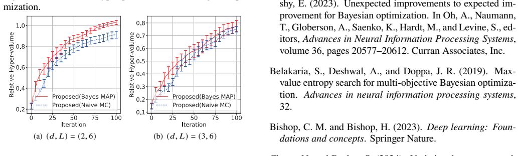
- [Section 3.3, Eq. (8); Section 6.4, Fig. 7; Appendix K.1] The variational lower-bound guarantee and the KL-minimization interpretation in Remark 3.1 apply to the naive Monte Carlo estimator Eq. (6), but all main experiments (Figs. 3-6 and the appendix results) use the biased MAP estimator Eq. (8), where I(f∈A^O) is replaced by θ_MAP=(p̂+I)/2. Eq. (8) is not guaranteed to be a lower bound on MI, as acknowledged in the text, while the mechanism claimed to improve performance (the mixture of over- and under-truncation) only affects Eq. (6). The only ablation, Fig. 7 and Appendix K.1, compares Eq. (8) with Eq. (6) within PFEV and shows that the MAP version performs considerably better; this makes the reported gains over PFES and {PF}2ES at L≥3 potentially attributable to the smoothing/bias of Eq. (8) rather than to the variational mixture. To support the paper's central claim, the authors should compare PFEV with Eq. (6) (or with a sufficiently large K unbiased estimate) against PFES and {PF}2ES on the same problems, and ideally also report the selected λ values and acquisition ordering for both estimators.
- [Appendix D.1; Section 3.3, Eq. (8)] The beta-prior approximation with mode at p̂=Z_O/Z_U and r=1 is an ad hoc heuristic that is not derived from the model: p̂ is the probability under the under-truncated distribution, not under the true conditioning on F*, so the prior mode can itself be substantially biased when the over- and under-truncated regions differ greatly (which the paper argues is the case for L≥3, see Fig. 2). The paper's justification for Eq. (8) is purely a variance-reduction argument, and the empirical evidence (Fig. 7 and Fig. 21) is based on average hypervolume, not on whether the estimator preserves the ranking of acquisition values across candidate points. A sensitivity analysis with respect to r, together with a direct comparison of the acquisition functions induced by Eq. (6) and Eq. (8), is needed to determine whether the observed benefit is due to the variational mixture or to the specific smoothing procedure.
minor comments (5)
- [Section 2] The notation "B" used to denote equality by definition (e.g., "𝒇 𝒙 B(...)") appears to be a formatting artifact and should be replaced with a standard symbol such as "≜" throughout.
- [Section 3.2, Eq. (3)] The set A^{U\O} is used in Eq. (3) but is formally defined only after the equation; it would be clearer to define A^{U\O} = A^U \ A^O just before the display.
- [Figure 1] The figure caption is dense and does not explain the meaning of the red star points, the dashed lines, or why the mixture is conceptually between the over- and under-truncated regions; a short explanation of each panel would improve readability.
- [References] The reference "Vlennet, R., Fonteix, C., and Marc, I." should be "Viennet" to match the standard spelling of the Viennet function.
- [Throughout] The paper uses "hyper-volume" and "hypervolume" interchangeably; please choose one spelling for consistency.
Circularity Check
No circularity: the variational lower-bound derivation is self-contained, lambda optimization is a genuine variational step, and empirical claims are benchmark-based; the Eq. (8) estimator concern is an experimental confound, not a circularity.
full rationale
The paper's derivation chain is self-contained. The mutual-information lower bound in Eq. (1) follows from the standard KL decomposition MI = LB + E[KL(true || variational)], and the variational distribution q_lambda is an explicit mixture of the under-truncated and over-truncated densities. Maximizing LB with respect to lambda in Eq. (5) is a legitimate variational minimization of the expected KL divergence to the true truncated posterior, as stated in Remark 3.1, and it is not a fit to the objective data that is later relabeled as a prediction. The only hand-chosen constants are the beta-prior strength r=1 and the 11-point lambda grid, both fixed across all problems, so there is no input-dependent fitted parameter masquerading as a result. The Eq. (8) MAP estimator replaces the indicator with theta_MAP = (p_hat + I)/2; this is a heuristic variance-reduction device, and the fact that all main experiments use it rather than the unbiased Eq. (6) is a legitimate experimental-attribution concern, not a circularity: the estimator is not constructed from the benchmark optima or from the reported hypervolume values. Citations to the authors' earlier works (Suzuki et al. 2020; Takeno et al. 2022) are used for the truncation idea and as baselines, but the load-bearing variational inequality is derived in the paper and in standard variational-inference references, so no self-citation chain forces the conclusion. The empirical comparisons are against external baselines on GP-generated functions, standard benchmarks, and hyperparameter optimization, and the reported advantage at L>=3 is an empirical outcome rather than an identity. No equation in the paper is equivalent to its own input by construction.
Assumptions & free parameters
free parameters (2)
- lambda =
optimized per (x, iteration) by maximizing LB(x,lambda)
- r (beta prior concentration) =
1
assumptions (4)
- domain assumption Each objective function is modeled by an independent Gaussian process with known kernel and Gaussian noise.
- domain assumption F*_S, obtained by NSGA-II on random feature map sample paths, is a finite subset of the true Pareto frontier F*.
- standard math The true conditional distribution p(f|F*) is supported within the under-truncation region A^U_{F*_S}.
- ad hoc to paper The beta prior with mode p̂ approximates the posterior of the probability θ = p(f∈A^O|F*).
Cite this review
Pith. "Pith review of Pareto-frontier Entropy Search with Variational Lower Bound Maximization." pith.science (2026). https://pith.science/paper/BIXHGGMO
@misc{pith2026250119073,
  author       = {Pith},
  title        = {Pith review of: Pareto-frontier Entropy Search with Variational Lower Bound Maximization},
  year         = {2026},
  howpublished = {\url{https://pith.science/paper/BIXHGGMO}},
  note         = {Machine review of arXiv:2501.19073}
}
read the original abstract
This study considers multi-objective Bayesian optimization (MOBO) through the information gain of the Pareto-frontier. To calculate the information gain, a predictive distribution conditioned on the Pareto-frontier plays a key role, which is defined as a distribution truncated by the Pareto-frontier. However, it is usually impossible to obtain the entire Pareto-frontier in a continuous domain, and therefore, the complete truncation cannot be known. We consider an approximation of the truncate distribution by using a mixture distribution consisting of two possible approximate truncation obtainable from a subset of the Pareto-frontier, which we call over- and under-truncation. Since the optimal balance of the mixture is unknown beforehand, we propose optimizing the balancing coefficient through the variational lower bound maximization framework, by which the approximation error of the information gain can be minimized. Our empirical evaluation demonstrates the effectiveness of the proposed method particularly when the number of objective functions is large.
Figures


Figures from the paper (26 more)




Reference graph
Works this paper leans on
-
[1]
Ament, S., Daulton, S., Eriksson, D., Balandat, M., and Bakshy, E. (2023). Unexpected improvements to expected improvement for B ayesian optimization. In Oh, A., Naumann, T., Globerson, A., Saenko, K., Hardt, M., and Levine, S., editors, Advances in Neural Information Processing Systems , volume 36, pages 20577--20612. Curran Associates, Inc
work page 2023
-
[2]
Belakaria, S., Deshwal, A., and Doppa, J. R. (2019). Max-value entropy search for multi-objective B ayesian optimization. Advances in neural information processing systems , 32
work page 2019
-
[3]
Bishop, C. M. and Bishop, H. (2023). Deep learning: Foundations and concepts . Springer Nature
work page 2023
-
[4]
Variational Entropy Search for Adjusting Expected Improvement
Cheng, N. and Becker, S. (2024). Variational entropy search for adjusting expected improvement. arXiv:2402.11345
work page Pith review arXiv 2024
-
[5]
Cover, T. M. and Thomas, J. A. (2006). Elements of Information Theory . Wiley-Interscience
work page 2006
-
[6]
Daulton, S., Balandat, M., and Bakshy, E. (2020). Differentiable expected hypervolume improvement for parallel multi-objective B ayesian optimization. In Larochelle, H., Ranzato, M., Hadsell, R., Balcan, M., and Lin, H., editors, Advances in NeuralInformation Processing Systems , volume 33, pages 9851--9864. Curran Associates, Inc
work page 2020
-
[7]
Daulton, S., Balandat, M., and Bakshy, E. (2021). Parallel B ayesian optimization of multiple noisy objectives with expected hypervolume improvement. In Ranzato, M., Beygelzimer, A., Dauphin, Y., Liang, P., and Vaughan, J. W., editors, Advances in NeuralInformation Processing Systems , volume 34, pages 2187--2200. Curran Associates, Inc
work page 2021
-
[8]
Daulton, S., Balandat, M., and Bakshy, E. (2023). Hypervolume knowledge gradient: A lookahead approach for multi-objective B ayesian optimization with partial information. In Proceedings of the 40th International Conference on Machine Learning , volume 202 of Proceedings of Machine Learning Research , pages 7167--7204. PMLR
work page 2023
Show all 42 references
-
[9]
Deb , K., Pratap , A., Agarwal , S., and Meyarivan , T. (2002). A fast and elitist multiobjective genetic algorithm: NSGA-II . IEEE Transactions on Evolutionary Computation , 6(2):182--197
2002
-
[10]
Emmerich, M. T. (2005). Single-and multi-objective evolutionary design optimization assisted by gaussian random field metamodels . PhD thesis, Dortmund University, Germany
2005
-
[11]
and Hern\' a ndez-Lobato, D
Fern\' a ndez-S\' a nchez, D. and Hern\' a ndez-Lobato, D. (2024). Joint entropy search for multi-objective B ayesian optimization with constraints and multiple fidelities. In ESANN 2024 proceedings, European Symposium on Artificial Neural Networks, Computational Intelligence ...
2024
-
[12]
E., Everson, R
Fieldsend, J. E., Everson, R. M., and Singh, S. (2003). Using unconstrained elite archives for multiobjective optimization. IEEE Transactions on Evolutionary Computation , 7(3):305--323
2003
-
[13]
Fonseca, C. M. and Fleming, P. J. (1995). Multiobjective genetic algorithms made easy: selection sharing and mating restriction. In First International Conference on Genetic Algorithms in Engineering Systems: Innovations and Applications , pages 45--52. IET
1995
-
[14]
GPy : A G aussian process framework in python
GPy (since 2012). GPy : A G aussian process framework in python. http://github.com/SheffieldML/GPy
2012
-
[15]
and Schuler, C
Hennig, P. and Schuler, C. J. (2012). Entropy search for information-efficient global optimization. Journal of Machine Learning Research , 13(57):1809--1837
2012
-
[16]
Hernandez-Lobato, D., Hernandez-Lobato, J., Shah, A., and Adams, R. (2016). Predictive entropy search for multi-objective B ayesian optimization. In Proceedings of The 33rd International Conference on Machine Learning , volume 48, pages 1492--1501. PMLR
2016
-
[17]
M., Hoffman, M
Hern\' a ndez-Lobato, J. M., Hoffman, M. W., and Ghahramani, Z. (2014). Predictive entropy search for efficient global optimization of black-box functions. In Advances in Neural Information Processing Systems 27 , page 918–926. Curran Associates, Inc
2014
-
[18]
R., Perttunen, C
Jones, D. R., Perttunen, C. D., and Stuckman, B. E. (1993). Lipschitzian optimization without the lipschitz constant. Journal of Optimization Theory and Applications , 79(1):157--181
1993
-
[19]
Kandasamy, K., Krishnamurthy, A., Schneider, J., and P \'o czos, B. (2018). Parallelised B ayesian optimisation via T hompson sampling. In Proceedings of the 21st International Conference on Artificial Intelligence and Statistics , volume 84, pages 133--142. PMLR
2018
-
[20]
Ke, G., Meng, Q., Finley, T., Wang, T., Chen, W., Ma, W., Ye, Q., and Liu, T.-Y. (2017). LightGBM : A highly efficient gradient boosting decision tree. Advances in neural information processing systems , 30
2017
-
[21]
Knowles, J. (2006). ParEGO : A hybrid algorithm with on-line landscape approximation for expensive multiobjective optimization problems. IEEE transactions on evolutionary computation , 10(1):50--66
2006
-
[22]
Kursawe, F. (1990). A variant of evolution strategies for vector optimization. In International conference on parallel problem solving from nature , pages 193--197. Springer
1990
-
[23]
Minka, T. P. (2001). Expectation propagation for approximate B ayesian inference. In Proceedings of the 17th Conference in Uncertainty in Artificial Intelligence , pages 362--369. Morgan Kaufmann Publishers Inc
2001
-
[24]
Ozaki, R., Ishikawa, K., Kanzaki, Y., Takeno, S., Takeuchi, I., and Karasuyama, M. (2024). Multi-objective B ayesian optimization with active preference learning. In Proceedings of the Thirty-Eighth AAAI Conference on Artificial Intelligence . AAAI Press
2024
-
[25]
Paria, B., Kandasamy, K., and P \'o czos, B. (2020). A flexible framework for multi-objective bayesian optimization using random scalarizations. In Uncertainty in Artificial Intelligence , pages 766--776. PMLR
2020
-
[26]
Perrone, V., Shcherbatyi, I., Jenatton, R., Archambeau, C., and Seeger, M. (2019). Constrained B ayesian optimization with max-value entropy search. arXiv:1910.07003
2019 arXiv
-
[27]
Picheny, V. (2015). Multiobjective optimization using gaussian process emulators via stepwise uncertainty reduction. Statistics and Computing , 25(6):1265--1280
2015
-
[28]
Ponweiser, W., Wagner, T., Biermann, D., and Vincze, M. (2008). Multiobjective optimization on a limited budget of evaluations using model-assisted-metric selection. In International conference on parallel problem solving from nature , pages 784--794. Springer
2008
-
[29]
B., Dhaene, T., and Couckuyt, I
Qing, J., Moss, H. B., Dhaene, T., and Couckuyt, I. (2022). \ PF \ ^2 ES : Parallel feasible pareto frontier entropy search for multi-objective B ayesian optimization. arXiv preprint arXiv:2204.05411
2022 arXiv
-
[30]
and Recht, B
Rahimi, A. and Recht, B. (2008). Random features for large-scale kernel machines. In Advances in Neural Information Processing Systems 20 , pages 1177--1184. Curran Associates, Inc
2008
-
[31]
Russo, L. M. and Francisco, A. P. (2014). Quick hypervolume. IEEE Transactions on Evolutionary Computation , 4(18):481--502
2014
-
[32]
and Ghahramani, Z
Shah, A. and Ghahramani, Z. (2016). Pareto frontier learning with expensive correlated objectives. In International conference on machine learning , pages 1919--1927. PMLR
2016
-
[33]
Shahriari, B., Swersky, K., Wang, Z., Adams, R., and De Freitas , N. (2016). Taking the human out of the loop: A review of B ayesian optimization. Proceedings of the IEEE , 104(1):148--175
2016
-
[34]
Srinivas, N., Krause, A., Kakade, S., and Seeger, M. (2010). Gaussian process optimization in the bandit setting: No regret and experimental design. In Proceedings of the 27th International Conference on International Conference on Machine Learning , pages 1015--1022. Omnipress
2010
-
[35]
Suzuki, S., Takeno, S., Tamura, T., Shitara, K., and Karasuyama, M. (2020). Multi-objective B ayesian optimization using P areto-frontier entropy. In Proceedings of the 37th International Conference on Machine Learning , volume 119, pages 9279--9288. PMLR
2020
-
[36]
Takeno, S., Fukuoka, H., Tsukada, Y., Koyama, T., Shiga, M., Takeuchi, I., and Karasuyama, M. (2020). Multi-fidelity B ayesian optimization with max-value entropy search and its parallelization. In Proceedings of the 37th International Conference on Machine Learning , volume 1...
2020
-
[37]
Takeno, S., Tamura, T., Shitara, K., and Karasuyama, M. (2022). Sequential and parallel constrained max-value entropy search via information lower bound. In Proceedings of the 39th International Conference on Machine Learning , volume 162 of Proceedings of Machine Learning Res...
2022
-
[38]
Tu, B., Gandy, A., Kantas, N., and Shafei, B. (2022). Joint entropy search for multi-objective B ayesian optimization. Advances in Neural Information Processing Systems , 35:9922--9938
2022
-
[39]
Vlennet, R., Fonteix, C., and Marc, I. (1996). Multicriteria optimization using a genetic algorithm for determining a pareto set. International Journal of Systems Science , 27(2):255--260
1996
-
[40]
and Jegelka, S
Wang, Z. and Jegelka, S. (2017). Max-value entropy search for efficient B ayesian optimization. In Proceedings of the 34th International Conference on Machine Learning , volume 70, pages 3627--3635. PMLR
2017
-
[41]
Zuluaga, M., Krause, A., et al. (2016). e-pal: An active learning approach to the multi-objective optimization problem. Journal of Machine Learning Research , 17(104):1--32
2016
-
[42]
Zuluaga, M., Sergent, G., Krause, A., and P \"u schel, M. (2013). Active learning for multi-objective optimization. In International conference on machine learning , pages 462--470. PMLR
2013
Reviewed August 9, 2026 · model on record in the stance chip above.
Discussion (0). Continue with ORCID to comment.