REVIEW 3 major objections 7 minor 3 references
Impermanent loss and Loss-vs-Rebalancing II
T0 review · 3 major / 7 minor · reviewed 2026-08-08 · deepseek-v4-flash
Pith's one-line read For a constant-product AMM, IL and LVR start identical, share one average at intermediate times, and separate at long times; fees suppress LVR far more than IL.
desk verdict Useful regime map and a genuinely new IL distribution, but the equal-average claim holds only for small sigma^2 T and the paper overstates its validity range. read the letter →
The pith
A machine-rendered reading of the paper's core claim, the machinery that carries it, and where it could break.
The reading
What carries the argument
The load-bearing object is the one-step identity $IL(p,p+dp)=L\sqrt{p}(1-\sqrt{p/(p+dp)})^2$, which is also the differential LVR; expanding for small moves gives $L\,dp^2/(4p^{5/2})$. Averaging this with the Brownian quadratic variation $dp^2=p^2\sigma^2\,dt$ produces the shared expectation $\langle IL\rangle=\langle LVR\rangle=L\sigma^2 T/(4\sqrt{p_0})$ in the intermediate regime. The distributional split comes from inverting IL as a function of the final price and applying the Jacobian $|dp/dIL|$, which yields the $1/\sqrt{IL}$ singularity, while the LVR distribution is recovered by summing many such draws in accordance with the central limit theorem. For fees, the machinery is the no-trade band $p(1-f)$ to $p/(1-f)$ and a first-passage random walk whose asymmetric barriers give $\langle N_{\mathrm{arb}}\rangle\propto f/(\sigma\sqrt{\Delta t})$, the characteristic arbitrage time that separates fee-dominated from fee-less behavior.
What would settle it
Simulate 100,000 geometric Brownian motion paths with $p_0=100$, $L=10000$, $\sigma=0.02$ over 2500 steps so that $\sigma^2 T=1$, and compare the empirical means of IL and LVR; if the means agree within statistical error, the paper's long-time divergence claim is wrong, since the paper predicts separation for $\sigma^2 T\ge 1$. A cheaper check is to evaluate the exact unexpanded integrals for $\langle IL\rangle$ and $\langle LVR\rangle$ under GBM at $\sigma^2 T=1$.
Extended reading notes
Core claim
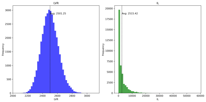
The paper's central claim is that, for a constant-product AMM whose price follows Brownian motion on short and intermediate horizons and geometric Brownian motion on long horizons and is arbitraged against an infinite-liquidity external market, IL and LVR are the same quantity only in the $\sigma^2 T\ll 1$ limit. In the intermediate regime $0\ll\sigma^2 T<1$, single-step IL and differential LVR coincide, and expanding that common expression to order $\Delta p^2$ gives $\Delta LVR\approx L\,\Delta p^2/(4p^{5/2})$. Because $\langle\Delta p^2\rangle=p^2\sigma^2\Delta t$, the two metrics share the average $L\sigma^2 T/(4\sqrt{p_0})$, which the paper derives analytically; yet their distributions are very different, with LVR a narrow central-limit-theorem sum and IL showing a $1/\sqrt{IL}$ singular pile-up near zero plus rare large-loss outliers. In the long-time regime $\sigma^2 T\ge 1$, geometric Brownian motion matters and even the averages separate, with LVR becoming log-normal-like while IL keeps its shape. Adding fees creates a no-trade band around the AMM price and introduces an average arbitrage time; the result is that fees cut average LVR far more than average IL, and can turn the net IL after fees positive for most paths without protecting against extreme IL.
Load-bearing premise
The paper's central equality of average IL and average LVR rests on the price staying close to its starting value, so that the expansion around $p\approx p_0$ is valid; the authors flag that this is only justified when $\sigma^2 T<1$.
Editorial extensions
If this is right
- For $\sigma^2 T<1$, both metrics have the same average $L\sigma^2T/(4\sqrt{p_0})$, growing linearly in time and quadratically in volatility, so statements about one average transfer to the other in this regime.
- Most price trajectories realize near-average LVR but below-average IL, so a typical LP position is better than its IL average yet close to its LVR average.
- Fees introduce a no-trade band and an arbitrage time scale; when the block time $\Delta t$ is small compared with $f/\sigma$, average LVR is suppressed from $\sigma^2 T$ scaling to $\sigma^3 T/(f\sqrt{\Delta t})$ and arbitrage volume changes from $\sigma\sqrt{TN}$ to $\sigma^2T/f$ scaling.
- At $\sigma^2 T\ge 1$, the equal-average statement fails and LVR's distribution becomes log-normal-like, so regime boundaries matter for any empirical comparison.
- Arbitrage volume over a fixed horizon grows like $\sqrt{N}$ with the number of steps, so the continuous-time limit is not well defined without a finite block time, fees, or tick spacing as a cutoff.
Reading between the lines
- I read the CLT construction as implying that LVR is a comparatively stable estimator of adverse-selection cost: averaging many pools should concentrate around the mean, whereas IL estimates remain sensitive to rare large moves, so risk reports should quote both.
- A direct extension the paper does not run is to add uninformed non-arbitrage traders; the no-trade band should survive, but fee revenue and LVR contributions would acquire additional terms and the optimal fee could shift from the pure-arbitrage value.
- Because the arbitrage-volume divergence is driven by $\sqrt{N}$ scaling, comparing AMMs across chains with different block times requires an explicit normalization; LVR per block rather than LVR per unit time may be the more portable quantity.
- The asymmetric-barrier result suggests a testable prediction for fee policy: the average time between arbitrages should grow linearly with $f/(\sigma\sqrt{\Delta t})$ in the fee-dominated regime, so doubling the fee should roughly double the expected time between arbitrage events rather than quadruple it.
Editorial analysis
A structured set of objections, weighed in public.
Referee Report
Summary. The paper studies the statistical relationship between impermanent loss (IL) and loss-versus-rebalancing (LVR) for constant-product AMMs under Brownian/geometric Brownian price dynamics. It proposes a three-regime classification in the dimensionless time sigma^2 T: a very short regime (IL is identical to LVR), an intermediate regime (distinct distribution functions but equal averages, with the LVR distribution obtained from the IL distribution via the central limit theorem), and a long regime (distinct averages and distributions). It further analyzes how transaction fees reduce average LVR much more strongly than average IL, and shows that arbitrage volume diverges as sqrt(N) in the continuous-time limit while the average inter-arbitrage time scales as f/(sigma sqrt(dt)). The analytic results are combined with Monte Carlo simulations throughout.
Significance. If correctly scoped, the paper offers a useful, accessible synthesis: an explicit closed-form distribution function for IL (Eq. 9) with its 1/sqrt(IL) small-IL singularity, a CLT-based explanation for the approximately Gaussian LVR distribution, falsifiable scaling predictions (the sqrt(N) volume divergence, the f/(sigma sqrt(dt)) scaling of the average inter-arbitrage time, and the fee-regime scalings of LVR and volume), and the observation that fees suppress average LVR far more than average IL. The distribution-function analysis appears to be the main new element relative to Milionis et al. and Fritsch et al., which the paper acknowledges. The Monte Carlo checks of the scaling laws are genuine numerical verifications of analytically predicted exponents rather than fitted parameters. However, the central quantitative claim (equal averages across the whole intermediate regime) is not supported beyond leading order, and the foundational definitions in Sec. 3.1 contain algebra and numeraire errors; a revision that repairs these would put the paper's claims on solid ground within a properly scoped regime.
major comments (3)
- [Sec. 4.2, Sec. 4.4, Table 1, App. B.2] The claim that <IL> = <LVR> throughout the intermediate regime (0 << sigma^2 T < 1, Table 1) is established only at leading order in sigma^2 T, and the paper's own assumptions do not cover the advertised range. The derivation replaces the running price by p0, and Sec. 4.2 states the underlying assumption that 'p does not change significantly over the time frame T, which is justified if sigma^2 T < 1.' That justification is too weak: relative price fluctuations are of order sqrt(sigma^2 T), so at sigma^2 T = 0.5-0.9 the expansion is not controlled, and the omitted corrections are of order (sigma^2 T)^2 and do not cancel. For zero-drift GBM in the continuum limit, using the paper's own IL formula (Eq. 4) and step-LVR formula of Sec. 3.2, one obtains <IL> = L sqrt(p0)(1 - 2 exp(3s/8) + exp(s)) and <LVR> = 2 L sqrt(p0)(1 - exp(-s/8)) with s = sigma^2 T; these agree only to order s/4 and differ by about (3/8) L sqrt(p0) s^2, roughly 60% of the leading term at s = 0.4. The paper's own Fig. 17 shows <IL(t)> departing from the linear law as t grows, and App. B.2 itself restricts the expansion to 'short times,' in tension with the unqualified wording of Table 1 and the abstract. Moreover, the GBM run in Fig. 6 (sigma = 0.02, 1000 steps) corresponds to total variance 0.4 under the paper's GBM update rule of Sec. 2.2.2, which is an intermediate-regime value by Table 1's criterion, yet the figure reports averages that 'differ significantly'; either the figure's parameters are misreported or the intermediate-regime equality fails at sigma^2 T = 0.4. No error bound is supplied anywhere. The authors should either compute the next-order corrections and show that they coincide, or re-scope the regime boundary and revise Table 1 and the abstract so that the equality is presented as the leading-order asymptote sigma^2 T -> 0.
- [Sec. 3.1, Eq. (4), App. C] The definition of IL contains algebra errors. The text asserts V(pf) = 2L sqrt(pf) = 2L sqrt(p) sqrt(p/pf), but 2L sqrt(p) sqrt(p/pf) = 2Lp/sqrt(pf), which is not equal to 2L sqrt(pf); and the HODL value is written as L sqrt(p)(1 + p/pf), whereas the correct y-denominated value is L sqrt(p)(1 + pf/p). Consequently Eq. (4), IL = L sqrt(p)(1 - sqrt(p/pf))^2, is not the exact HODL-minus-position loss. For a price doubling, Eq. (4) gives 0.0858 L sqrt(p) instead of the true 0.1716 L sqrt(p), and for pf -> infinity it saturates at L sqrt(p) while the true loss grows as L pf / sqrt(p). The 'exact' inversion used in App. C (Eqs. 30-32) and the long-time statements inherit this error. The leading-order expansions are unaffected, since both forms reduce to L (Delta p)^2 / (4 p^{3/2}), so the small-sigma^2 T results survive, but the paper should either correct the definition of IL or explicitly state that Eq. (4) is the leading-order (step-wise) loss, and then recompute the exact distribution function and the long-time behavior accordingly.
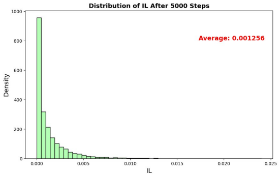
- [Sec. 4.2, App. A, App. B] There is an unstated numeraire inconsistency. The exact step-LVR formula in Sec. 3.2, L sqrt(p)(1 - sqrt(p/(p+dp)))^2, expands to L dp^2 / (4 p^{3/2}), but Sec. 4.2 and App. A claim the expansion L dp^2 / (4 p^{5/2}), a factor p smaller. For p = 100, dp = 1, L = 1000 the exact value is 0.2463, while the two expansions give 0.25 and 0.0025. The p^{5/2} form corresponds to denominating LVR in units of the x token (prefactor x0 = L/sqrt(p)), and App. B indeed uses that convention consistently: the quoted prediction <IL(5000)> = <LVR(5000)> = 0.00125 for x0 = 100, sigma0 = 0.01, t = 5000 is x0 sigma0^2 t / (4 p0^2), and Eq. (13) matches it. But Sec. 3.1's V and HODL are y-denominated, so the quantitative anchors of the paper differ by a factor p0 depending on which section one reads; under the y-denominated HODL-minus-V definition the average is p0 times larger (0.125). Note that the apparent factor-p0^2 discrepancy between Eq. (13) and App. B.2 disappears once one sets sigma0 = p0 sigma and L = x0 sqrt(p0); the real problem is that these identifications are never stated and Sec. 3.1 is internally inconsistent. The paper should fix one numeraire, state it explicitly, and propagate it through Eqs. (5), (6), (13), and (24)-(29).
minor comments (7)
- [Sec. 2.2 and App. B.2] The appendix's Gaussian density has variance sigma0^2 t, which corresponds to sigma0 = p0 sigma of the main text, but this identification is never stated, and sigma and sigma0 are used without distinction across Secs. 2, 4, and the appendices.
- [Sec. 4.3 and Table 1] The long-time regime boundary is quoted inconsistently: the abstract and Table 1 use sigma^2 T >= 1, while Sec. 4.3 writes sigma^2 T > 1.
- [Fig. 6 caption] The caption is incomplete ('1000 recorded over 10000 runs' should presumably read '1000 steps recorded over 10000 runs'), and with the stated parameters the run has total variance 0.4, which falls in the intermediate regime of Table 1; the figure's role as evidence for the long-time regime must be clarified.
- [Fig. 5 and Fig. 7 captions] Fig. 7's caption says 'l.h.s' twice, and Fig. 5's body text mentions 5000 samples while the caption text mentions 10000 samples.
- [Throughout] Several typos should be corrected: 'pratical', 'introducung', 'rice evolution', 'Feynamn', 'manged', 'V ariance', 'coring rules' (Hanson's paper is on scoring rules), and 'now-arbitrage zone'.
- [Eq. (12) and Sec. 4.3] The constants a and c in Eq. (12) are never specified, and the claim in Sec. 4.3 about 'the belief in the literature' that sums of truncated power-law random variables produce approximate log-normal distributions lacks a citation.
- [Eq. (7)] Eq. (7) writes <Delta P^2> = p^2 sigma^2 T without indicating that the prefactor is the initial price p0; the notation 'p2 sigma 2T' is confusing.
Circularity Check
No significant circularity: the central IL/LVR results are derived from the model definitions and explicit Gaussian integrals, not from fitted inputs; the main caveat is a small-σ²T approximation, which is a correctness-scope issue rather than a circular step.
full rationale
The paper's central derivation chain is self-contained. IL and LVR are defined by distinct formulas (Eq. 4 and the delta-LVR expression in Sec. 3.2), and the short-time identity is an algebraic equality of those definitions, not an input. In the intermediate regime, the equality of averages is obtained by expanding Gaussian Brownian-motion integrals in App. B.2: Eq. (27) and Eq. (29) both evaluate to x0σ0²t/(4p0²) using the same lowest-order expansion around p0, which is a calculation rather than a fitted or renamed quantity. The CLT construction of the LVR distribution in Sec. 4.2.1 is a Monte Carlo demonstration: the per-step identity is explicitly stated, and the sum-of-IL distribution is then simulated, so the Gaussian shape is a numerical finding rather than a parameter forced by construction. The fee-related scaling in Sec. 5 is fit to simulations of the same random-walk model that motivates the scaling; it is a numerical corroboration, not a parameter tuned to force an independent conclusion. The self-citations, including the sequel reference to Paper I, are contextual and non-load-bearing: no external uniqueness theorem or model choice is imported solely from the authors' prior work. The genuine weakness is a scope limitation, not circularity: the paper explicitly states that the average-equality expansion assumes p does not change significantly over T (Sec. 4.2), and App. B.2 calls the expansion 'short times' and shows a numerical solution that deviates from the linear law. This means the regime label 0≪σ²T<1 is overbroad without a quantified error bound, but overbreadth is a correctness concern, not a circular reduction. Score 2 reflects the presence of non-load-bearing self-citation, not a circular derivation.
Assumptions & free parameters
free parameters (1)
- power-law exponent b for (N_arb) scaling =
0.990 +/- 0.016
assumptions (5)
- domain assumption Price follows geometric Brownian motion (or Brownian motion) with zero drift and constant volatility sigma.
- domain assumption Constant-product AMM with xy = L^2 and no other trading activity besides arbitrage.
- ad hoc to paper The small-dp expansion IL = L dp^2 / (4 p^{5/2}) is valid and p stays near p0 over the horizon T, so averages can be evaluated with p approximately p0.
- domain assumption BM and GBM are equivalent for intermediate times (sigma^2 T < 1), so Gaussian price densities are used for IL distribution functions.
- standard math The central limit theorem applies to the sum of per-step LVR increments, so the LVR distribution is Gaussian.
Cite this review
Pith. "Pith review of Impermanent loss and Loss-vs-Rebalancing II." pith.science (2026). https://pith.science/paper/6QOKT2DV
@misc{pith2026250204097,
  author       = {Pith},
  title        = {Pith review of: Impermanent loss and Loss-vs-Rebalancing II},
  year         = {2026},
  howpublished = {\url{https://pith.science/paper/6QOKT2DV}},
  note         = {Machine review of arXiv:2502.04097}
}
read the original abstract
This paper examines the relationship between impermanent loss (IL) and loss-versus-rebalancing (LVR) in automated market makers (AMMs). Our main focus is on statistical properties, the impact of fees, the role of block times, and, related to the latter, the continuous time limit. We find there are three relevant regimes: (i) very short times where LVR and IL are identical; (ii) intermediate time where LVR and IL show distinct distribution functions but are connected via the central limit theorem exhibiting the same expectation value; (iii) long time behavior where both the distribution functions and averages are distinct. Subsequently, we study how fees change this dynamics with a special focus on competing time scales like block times and 'arbitrage times'.
Figures


Figures from the paper (15 more)




Reference graph
Works this paper leans on
-
[3]
Applied Mathematical Finance 30 30, 2 (2023), 69–93
Predictable Losses of Liquidity Provision in Constant Function Mar- kets and Concentrated Liquidity Markets. Applied Mathematical Finance 30 30, 2 (2023), 69–93. https://doi.org/10.1080/1350486X.2023.2277957 arXiv:https://doi.org/10.1080/1350486X.2023.2277957 31 A Differential equation for L VR While IL only cares about the start and end points of the pri...
-
[2021]
Optimal Fees for Geometric Mean Market Makers
Automatic market-making with dynamic peg . Retrieved Sept 18, 2023 from https://classic.curve.fi/files/crypto-pools-paper.pdf [Elsts(2024)] Atis Elsts. 2024. CEX/DEX arbitrage, transaction fees, block times, and LP profits . https://ethresear.ch/t/ cex-dex-arbitrage-transaction-fees-block-times-and-lp-profits/19444 29 [Evans et al.(2021)] Alex Evans, Guil...
work page Pith review arXiv 2024
-
[2023]
arXiv preprint arXiv:2305.14604 (2023)
Automated Market Making and Arbitrage Profits in the Presence of Fees. arXiv preprint arXiv:2305.14604 (2023). [Milionis et al.(2024)] Jason Milionis, Ciamac C. Moallemi, Tim Roughgarden, and Anthony Lee Zhang. 2024. Automated Market Making and Loss-Versus- Rebalancing. arXiv:2208.06046 [q-fin.MF] [MountainFarmer et al.(2022)] MountainFarmer, Louis, Hanzo...
arXiv 2023
Reviewed August 8, 2026 · model on record in the stance chip above.
Discussion (0). Continue with ORCID to comment.