REVIEW 3 major objections 4 minor 4 cited by
Linear Bandits with Partially Observable Features
T0 review · 3 major / 4 minor · reviewed 2026-08-08 · deepseek-v4-flash
Pith's one-line read Partial observability need not force linear regret in linear bandits.
desk verdict Fresh setting and a neat reparameterization, but the doubly robust estimator is biased under the resampling-until-match coupling, so the main regret bound does not follow from the proof. read the letter →
The pith
A machine-rendered reading of the paper's core claim, the machinery that carries it, and where it could break.
The reading
What carries the argument
The mechanism is projection and feature augmentation. The reward vector $Y$ is decomposed as $X^\top \theta^{(o)}_\star + U^\top \theta^{(u)}_\star$; projecting onto the row space $R(X)$ and its orthogonal complement $R(X)^\perp$ gives $X^\top \mu^{(o)}_\star + B^\top \mu^{(u)}_\star$, where $B$ is an orthonormal basis of $R(X)^\perp$. Augmenting each observed feature $x_a$ to $\tilde{x}_a = [x_a; e_a^\top B]$ makes every reward exactly linear in $\tilde{x}_a$ with parameter $\mu$, whose $\mu^{(u)}$ block has only $d_h$ nonzero entries. A doubly robust Lasso estimator with pseudo-rewards, coupled resampling, and inverse probability weights bounded by $O(K)$ turns this into an efficiently learnable sparse linear bandit.
What would settle it
Run RoLF on the two-arm instance from Theorem 1—observed features 1 and 2, unobserved features 3 and 19/4, true parameter $(2, -1)$, optimal arm 2—for a long horizon; if cumulative regret grows linearly instead of roughly $\sqrt{T}$, the central bound is false.
Extended reading notes
Core claim
The paper's central claim is that partial observability does not have to force linear regret. Because the reward is linear in the full vector $(x_a, u_a)$, the vector of expected rewards across all arms can be split by the projection onto the row space of the observed features and the projection onto its orthogonal complement; augmenting each observed feature with an orthonormal basis of that complement rewrites every arm's reward as a dot product $\tilde{x}_a^\top \mu$ with no extra misspecification term. The corresponding parameter $\mu$ is sparse outside the observed block, with $d_h$ nonzero coordinates, and a doubly robust Lasso estimator that imputes unselected arms' rewards makes all $K$ reward estimates converge at rate $\sqrt{(d + d_h)/t}$ (Theorem 2). RoLF then achieves cumulative regret $\tilde{O}(\sqrt{(d + d_h)T})$ with high probability (Theorem 3), while knowing neither $d_u$ nor $d_h$; the paper further shows that OFUL and LinTS suffer linear regret on a two-arm instance and that any policy depending only on observed features has a worst-case lower bound linear in $T$.
Load-bearing premise
The unobserved features must be fixed over time and the reward must be exactly linear in them; if the hidden reward component is nonlinear or drifts with time, the projection used to rewrite the problem as a sparse linear bandit breaks down.
Editorial extensions
If this is right
- Algorithms that use only observed features—OFUL, LinTS, LinUCB—can be made robust to latent features without modeling or recovering them, eliminating a source of linear regret.
- RoLF's regret is at most $\tilde{O}(\sqrt{(d + d_h)T})$, which is never worse than the $\tilde{O}(\sqrt{KT})$ regret of ignoring features entirely, since $d + d_h \le K$.
- When the latent feature space lies inside the observed row space, $d_h = 0$ and the bound becomes $\tilde{O}(\sqrt{dT})$, matching standard linear bandit performance despite hidden features.
- For time-varying observed features with fixed unobserved features, augmenting with the standard basis yields a $\tilde{O}(\sqrt{(d + K)T})$ bound, extending the approach to a setting where feature-ignoring algorithms would suffer linear regret.
- The algorithm requires no prior knowledge of the unobserved feature dimension or the sparsity level $d_h$, so it works even if more features become hidden over time.
Reading between the lines
- A corollary the paper does not spell out is that the same augmentation makes the hidden-feature gap visible: running RoLF on a problem where the latent reward is nonlinear should produce regret that grows with the projection error, so the algorithm could double as a diagnostic for whether linearity in the latent features holds.
- If the projection trick extends to generalized linear or nonparametric rewards, the sparse structure of $\mu$ in the augmented space would let practitioners reuse any high-dimensional bandit algorithm that needs only a sparse parameter, rather than a bespoke latent-feature estimator.
- One could test the tightness of the $d_h$ dependence by fixing $d$ and $K$ while rotating the relative orientation of the observed and unobserved feature spaces; the regret slope should increase smoothly with $d_h$, a prediction the paper's Case 1–3 experiments only partially probe.
Editorial analysis
A structured set of objections, weighed in public.
Referee Report
Summary. The paper studies fixed-action stochastic linear bandits in which the reward is linear in a full feature vector z_a=(x_a,u_a) but only the observed part x_a is available to the learner. The authors project the reward onto the row space of the observed features and its orthogonal complement, augment each observed feature with an orthonormal basis of the complement, and reparameterize the problem as a linear bandit in K-dimensional augmented features with a sparse parameter whose effective support size is d+d_h (Section 4.1). They then propose an algorithm, RoLF (Algorithm 1), that combines forced exploration, epsilon-greedy action selection, a resampling/coupling procedure for a pseudo-action, a Lasso imputation estimator, and a doubly robust Lasso estimator. The main claim is Theorem 3: with high probability the cumulative regret is O~(sqrt((d+d_h)T)), without the algorithm knowing d_h or the unobserved feature space. The paper also gives a linear-regret lower bound for OFUL and LinTS that ignore latent features (Theorem 1), an extension to time-varying observed features (Appendix D), and numerical experiments.
Significance. The problem is well motivated and the algebraic projection in Eqs. (4)-(7) is a clean idea: it removes the explicit misspecification term and converts the latent-feature issue into sparsity of the projected reward in an augmented basis. If the main theorem were correct, it would be a genuine advance over prior work that assumes Gaussian or dynamically evolving latent features. The paper also provides a simple lower-bound instance for algorithms that ignore the latent component, and the experimental section is reasonably broad. The weakness is that the central proof mechanism, the unbiasedness of the doubly robust pseudo-rewards, is not valid for the algorithm as written: the proof relies on a distribution of pseudo-actions that the matched-sampling loop of Algorithm 1 never actually uses. Since Theorems 2 and 3 depend on this unbiasedness, the paper's central claim is not established.
major comments (3)
- [Sec. 4.2, Eq. (10); Algorithm 1, lines 10-20] The pseudo-reward estimator is not unbiased under the algorithm's matched-sampling rule. In the only rounds used by Eq. (11), the resampling loop has terminated with e_t=a_t, so I(e_t=a)=I(a_t=a) for every a. For a different from a_t the correction term is zero, and for a=a_t the denominator is p. Hence E[\tilde{y}_{a,t}|F_{t-1}] = \tilde{x}_a^\top \check{\mu}_t + (P(a_t=a)/p)(\tilde{x}_a^\top \mu^* - \tilde{x}_a^\top \check{\mu}_t). The action probability P(a_t=a) is 1-t^{-1/2} for the greedy candidate and t^{-1/2}/(K-1) for the others, while p is a fixed constant in (1/2,1), so this equals the true mean only in the unattainable case P(a_t=a)=p. The text's claim that taking expectation over e_t gives unbiasedness is therefore invalid: e_t is sampled conditionally on a_t and the update is conditioned on the event M_t. This bias invalidates the martingale condition E[I(e_\tau=a)/\phi_{a,\tau}-1|F_{\tau-1}]=0 that underpins Theorem 2 and Theorem 3. A related issue is that Eq. (10) is formally undefined when e_t=a and a\neq a_t, because y_{a,t} is not observed; the algorithm avoids this by discarding unmatched rounds, but that is precisely the conditioning that creates the bias.
- [Appendix G.2, Corollary 1; proof of Theorem 2 in Appendix E.2] The claimed concentration A_t\approx V_t is inconsistent with Algorithm 1. The martingale calculation in Corollary 1 uses the law of e_t in Eq. (9) conditional on a_t, under which e_t can equal an arm different from a_t and E[I(e_t=a)/\phi_{a,t}|a_t]=1 for every a. But every sample entering the estimator in Eq. (11) satisfies e_t=a_t; on the high-probability event that M_\tau holds for all \tau, A_t=(1/p)\sum_{\tau}\tilde{x}_{a_\tau}\tilde{x}_{a_\tau}^\top. Its conditional increment has expectation (1/p)\sum_a P(a_\tau=a)\tilde{x}_a\tilde{x}_a^\top, which is not the increment V_t increment \sum_a\tilde{x}_a\tilde{x}_a^\top. The bound (23), and hence the lower bound on \lambda_{\min}(A_t) used in the proof of Theorem 2, is therefore unavailable. Since Theorem 3 is derived from Theorem 2, the regret bound does not follow from the provided arguments.
- [Appendix E.2 and Sec. 4.2] There is an additional eigenvalue gap in the Lasso imputation argument. The imputation estimator \check{\mu}_t in Eq. (8) is fit only to the chosen actions. Lemma 3 bounds \|\check{\mu}_t-\mu^*\|_{\Sigma_t} in terms of \lambda_{\min}(\Sigma_t), where \Sigma_t is the selected-action Gram matrix. With |E_t|=O(K^3\log(T/\delta)) forced-uniform rounds and the remaining rounds concentrating on the greedy arm, \lambda_{\min}(\Sigma_t) is O(\log t), not \Omega(t). The proof substitutes A_t for \Sigma_t and uses \lambda_{\min}(A_t)\ge(1-\epsilon)\lambda_{\min}(V_t), but under matched sampling A_t=(1/p)\Sigma_t, so this substitution would require the selected-action Gram to be close to the full K-action Gram. That is impossible for an epsilon-greedy action distribution with p\in(1/2,1). Thus the consistency rate in Theorem 2 and the resulting regret bound in Theorem 3 are not supported.
minor comments (4)
- [Sec. 4.1] The sentence 'when K>d and du=0, the regret is the regret is higher than that of OLB algorithms' contains a duplicated phrase and should be rewritten.
- [Algorithm 1, line 6] The pseudocode says 'Randomly sample b_hat uniformly over [K]'; because line 11 randomizes a_t around b_hat, the marginal law of a_t in exploration rounds is indeed uniform, but the pseudocode should state this explicitly to avoid appearing to contradict the text in Section 4.2.
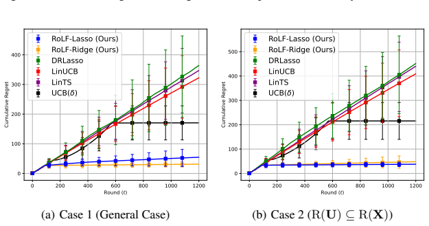
- [Sec. 6] For the reported K=30, the exploration factor C_e=(8K)^3\tilde{\sigma}_{\min}^{-2}\tilde{\sigma}_{\max}^2(1-p)^{-2} is on the order of 10^7, far exceeding the horizon T=1200 used in the experiments. The experiments are therefore entirely within the forced-exploration phase and do not test the post-exploration behavior described by Theorem 3.
- [Appendix D, Theorem 6] The proof of Theorem 6 is omitted with the statement that it 'follows similar arguments.' Since the time-varying setting changes the augmented feature vectors every round and the Gram matrices are no longer constant, the extension is not immediate and should either be proved or explicitly presented as a conjecture.
Circularity Check
No circularity: the regret bound is a conditional upper bound in terms of a problem-defined sparsity d_h, and the algorithm does not fit or tune d_h.
full rationale
The central derivation is self-contained: Eq. (4) is an algebraic identity that rewrites the reward vector using projections onto the row space of observed features and its orthogonal complement, and Eq. (7) simply expresses the same reward with augmented features. The quantity d_h in Eq. (6) is defined as the number of nonzero coefficients of the projected latent reward in a fixed orthonormal basis; the bound in Theorem 3 is stated for any delta and p in terms of this fixed problem parameter, and Algorithm 1 does not observe, estimate, or tune d_h. Thus the regret bound is a genuine conditional upper bound rather than a renamed input. The DR pseudo-reward construction is inspired by prior self-citations (Kim et al., 2021, 2023c), but the novel consistency argument (Theorem 2) is proved in Appendix E.2, and the Lasso error bound used in that proof (Lemma 3) is proved in Appendix G.3 despite being inspired by Lemma B.4 of Kim et al. (2024). No uniqueness theorem from the authors' prior work is invoked to force the choice of algorithm, and no fitted parameter is relabeled as a prediction. The skeptic's objection about the unbiasedness of the pseudo-rewards under the coupling event M_t is a correctness concern about the martingale argument, not a circularity: biasedness of an estimator is not an equivalence between the theorem and its assumptions. The paper explicitly notes that arbitrarily varying latent features make the problem non-learnable, which is a stated assumption rather than a hidden circular step. The omitted proof of Theorem 6 in Appendix D.2 is a completeness gap but not a circularity.
Assumptions & free parameters
free parameters (2)
- coupling probability p =
0.6 in experiments
- confidence parameter delta =
1e-4 in experiments
assumptions (4)
- domain assumption Reward is exactly linear in the full arm feature vector: y_{a,t} = <z_a, theta*> + epsilon_t (Eq. 2).
- domain assumption Noise is conditionally sigma-sub-Gaussian (Assumption 1).
- domain assumption Observed and unobserved features are fixed over time.
- domain assumption The observed feature vectors span R^d (or are reduced by SVD to a full-row-rank matrix).
Cite this review
Pith. "Pith review of Linear Bandits with Partially Observable Features." pith.science (2026). https://pith.science/paper/7PKAJ4RN
@misc{pith2026250206142,
  author       = {Pith},
  title        = {Pith review of: Linear Bandits with Partially Observable Features},
  year         = {2026},
  howpublished = {\url{https://pith.science/paper/7PKAJ4RN}},
  note         = {Machine review of arXiv:2502.06142}
}
abstract
We study the linear bandit problem that accounts for partially observable features. Without proper handling, unobserved features can lead to linear regret in the decision horizon $T$, as their influence on rewards is unknown. To tackle this challenge, we propose a novel theoretical framework and an algorithm with sublinear regret guarantees. The core of our algorithm consists of (i) feature augmentation, by appending basis vectors that are orthogonal to the row space of the observed features; and (ii) the introduction of a doubly robust estimator. Our approach achieves a regret bound of $\tilde{O}(\sqrt{(d + d_h)T})$, where $d$ is the dimension of the observed features and $d_h$ depends on the extent to which the unobserved feature space is contained in the observed one, thereby capturing the intrinsic difficulty of the problem. Notably, our algorithm requires no prior knowledge of the unobserved feature space, which may expand as more features become hidden. Numerical experiments confirm that our algorithm outperforms both non-contextual multi-armed bandits and linear bandit algorithms depending solely on observed features.
Figures

Forward citations
Cited by 4 Pith papers
-
Optimizing the Preconditioner: A Black-box Online-to-Nonconvex Conversion with Static Regret Minimization Oracles
An OCO algorithm with only O(√T) static regret, pluggable as a preconditioner selector, recovers the classical O(1/√T) stationarity rate on smooth stochastic nonconvex problems and the O(T^{-2/7}) rate on nonsmooth ones.
-
Stochastic Linear Bandits with Partially Observed Actions
TOFU-POV recovers a latent action subspace from randomly masked features and achieves √T regret scaling with intrinsic dimension m rather than ambient dimension d.
-
Pre-Trained AI Model Assisted Online Decision-Making under Missing Covariates: A Theoretical Perspective
The paper introduces model elasticity to bound the regret of contextual bandits with AI-imputed missing covariates, and shows that MAR-based calibration removes the dominant linear regret term.
-
Deconfounded Warm-Start Thompson Sampling with Applications to Precision Medicine
DWTS debiases and selects features from observational data, then warm-starts Thompson sampling with those estimates, achieving lower cumulative regret than LinTS in simulations.
Reference graph
Works this paper leans on
-
[1]
Rearranging terms gives V1/2 t A−1 t V1/2 t ⪯ (1 − ϵ)−1IK. Combining this with Eq. (29), max a∈[K] |ex⊤ a (bµR t − µ⋆)| ≤ maxa∈[K] ∥exa∥V−1 t 1 − ϵ tX τ =1 1 p exaτ ϵτ − µ⋆ V−1 t ≤ maxa∈[K] ∥exa∥V−1 t 1 − ϵ 1 p tX τ =1 exaτ ϵτ V−1 t + ∥µ⋆∥V−1 t , where the last inequality follows from the triangle inequality. Note thatVt is deterministic, both Vt ...
work page 2011
-
[2]
Given the true feature set Z = {[1, 3]⊤, [2, 19/4]⊤}, let the first element of each vector is observed to the agent; while the second element remains unobserved. This results in x1 = x1 = 1, x2 = x2 = 2, u1 = u1 = 3 and u2 = u2 = 19/4. We set the true parameter as θ⋆ ∈ R2 = [2, −1]⊤, meaning θ(o) ⋆ = θ(o) ⋆ = 2 and θ(u) ⋆ = θ(u) ⋆ = −1. Using the reward f...
work page 2017
-
[8]
and OFUL (Abbasi-yadkori et al., 2011), which are known for their practicality and performance guarantees. However, existing approaches differ from ours in two key aspects: (i) they assume that the learning agent can observe the entire feature vector related to the reward, and (ii) their algorithms have regret that scales linearly with the dimension of th...
work page 2019
-
[10]
(2023a) leverage a Bayesian oracle strategy for estimation; and Zeng et al
introduce a known decoder mapping from the observed features to the corresponding latent features; Kim et al. (2023a) leverage a Bayesian oracle strategy for estimation; and Zeng et al. (2025) estimate the true features using a Kalman filter. In contrast, our setting imposes no structural assumptions on either the observed or latent features, making the p...
work page 2023
-
[12]
(18) Since the second term of Eq
≤ exp − t 128σ2 + P(eθt ≥ 0 | bθt < 0). (18) Since the second term of Eq. (18) is calculated under a Gaussian distribution, thus its value does not exceed 1/2 for all t ∈ [T ], it follows that P(Ec eθ) ≥ 1/2 − exp −t/128σ2 . Note that the total decision horizon T >256σ2 log(1/δ′), thus 18 Linear Bandits with Partially Observable Features for any t >128σ2 ...
work page 2017
-
[14]
exp ( vλmax tX τ =1 Dτ !)# ≤ E
Let {Mτ : τ ∈ [t]} be a Rd×d-valued stochastic process adapted to the filtration {Fτ : τ ∈ [t]}, i.e., Mτ is Fτ - measurable for τ ∈ [t]. Suppose that the matrix Mτ is symmetric and the eigenvalues of the difference Mτ − E[Mτ |F τ −1] lie in [−b, b] for some b >0. Then for x >0, P tX τ =1 Mτ − E[Mτ |F τ −1] 2 ≥ x ! ≤ 2d exp − x2 2tb2 . Proof. The proof ad...
work page 2012
-
[15]
and t ≥ 8ϵ−2(1 − p)−2K 2 log(2Kt 2/δ), with probability at least 1 − δ/t2, IK − V−1/2 t AtV−1/2 t 2 ≤ ϵ. Proof. Note that V−1/2 t AtV−1/2 t − IK = V−1/2 t tX τ =1 X a∈[K] I(eaτ = a) ϕa,τ − 1 exaex⊤ a V−1/2 t , and the martingale difference matrix for each τ ∈ [t], X a∈[K] I(eaτ = a) ϕa,τ − 1 V−1/2 t exaex⊤ a V−1/2 t 2 ≤ X a∈[K] I(eaτ = a) ...
work page 2024
-
[1985]
employ the Upper Confidence Bound (UCB) strategy, which encourages the learner to select actions with the highest sum of estimated reward and uncertainty. This approach adaptively balances exploration and exploitation, and has been widely and studied in the context of linear bandits (Abe & Long, 1999; Auer, 2002; Dani et al., 2008; Rusmevichientong & Tsit...
work page 1999
Show all 15 references
-
[2009]
Partially observable contextual bandits with linear payoffs
11 Linear Bandits with Partially Observable Features Zeng, S., Bhatt, S., Koppel, A., and Ganesh, S. Partially observable contextual bandits with linear payoffs. In ICASSP 2025 - 2025 IEEE International Conference on Acoustics, Speech and Signal Processing (ICASSP),
2025
-
[2011]
Dani, V ., 9, ., Hayes, T., and Kakade, S. M. Stochastic linear optimization under bandit feedback. 21st Annual Conference on Learning Theory - COLT 2008, Helsinki, Finland, pp. 355–366,
2008
-
[2020]
and Faradonbeh, M
Park, H. and Faradonbeh, M. K. S. A regret bound for greedy partially observed stochastic contextual bandits. In Decision Awareness in Reinforcement Learning Workshop at ICML 2022,
2022
-
[2021]
Linear bandits with feature feedback
Oswal, U., Bhargava, A., and Nowak, R. Linear bandits with feature feedback. In The Thirty-Fourth AAAI Conference on Artificial Intelligence, AAAI 2020, The Thirty-Second Innovative Applications of Artificial Intelligence Confer- ence, IAAI 2020, The Tenth AAAI Symposium on Ed...
2020
-
[2022]
and Faradonbeh, M
Park, H. and Faradonbeh, M. K. S. Thompson sampling in partially observable contextual bandits. arXiv preprint arXiv:2402.10289,
-
[2024]
(2025) construct the observed features as emissions from the true features via a known linear mapping, also corrupted by additive Gaussian noise, whereas Kim et al
and Zeng et al. (2025) construct the observed features as emissions from the true features via a known linear mapping, also corrupted by additive Gaussian noise, whereas Kim et al. (2023a) first corrupt the true features with Gaussian noise and then generate the observed featu...
2025
-
[2025]
Related Works In bandit problems, the learning agent learns only from the outcomes of chosen actions, leaving unchosen alternatives unknown (Robbins, 1952)
12 Linear Bandits with Partially Observable Features A. Related Works In bandit problems, the learning agent learns only from the outcomes of chosen actions, leaving unchosen alternatives unknown (Robbins, 1952). This constraint requires a balance between exploring new actions...
1952
Reviewed August 8, 2026 · model on record in the stance chip above.
Discussion (0). Continue with ORCID to comment.