REVIEW 2 major objections 7 minor 58 references
A numerical analysis of Araki-Uhlmann relative entropy in Quantum Field Theory
T0 review · 2 major / 7 minor · reviewed 2026-08-07 · deepseek-v4-flash
Pith's one-line read For a free massive scalar field, the Araki-Uhlmann relative entropy between a coherent state and the vacuum decreases with mass and increases with the size of the region supporting the state.
desk verdict A clean standard derivation wrapped in a numerical scan whose central new claim is credible but rests on 10^8-point QMC with no convergence diagnostics. read the letter →
The pith
A machine-rendered reading of the paper's core claim, the machinery that carries it, and where it could break.
The reading
What carries the argument
The central object is the Araki-Uhlmann relative entropy $S(\Psi|\Omega) = -\langle\Psi|\log\Delta_{\Psi|\Omega}|\Psi\rangle$, defined through the relative Tomita-Takesaki modular operator $\Delta_{\Psi|\Omega}$. For coherent states the vacuum modular flow, given by the Bisognano-Wichmann boost action $\Delta^{is}_\Omega A_f \Delta^{-is}_\Omega = A_{\delta^{is} f}$, reduces the entropy to the smeared Pauli-Jordan expression $S(\Psi|\Omega) = -\frac{1}{2}\Delta_{PJ}(f, f'_s|_{s=0})$, which is the starting point of the computation. The numerical machinery is the four-dimensional quasi-Monte-Carlo integration of $J(m,\alpha)$ in Eq. (25), carried out for four test-function profiles localized in the right Rindler wedge.
What would settle it
Recompute the integral in Eq. (25) with an independent deterministic quadrature and with the sampling points varied by orders of magnitude, and check whether the derivatives $dS/dm$ and $dS/d\alpha$ keep the same sign and stabilize; if any monotonic curve reverses or changes shape as resolution increases, the central claim fails. An analytic evaluation for a test function with a known Fourier transform would give a sharp cross-check of the mass dependence.
Extended reading notes
Core claim
The paper's central claim is that for a coherent state $\Psi = A_f \Omega$ built from a test function $f$ supported in the right Rindler wedge of a free massive scalar field in $1+1$ Minkowski spacetime, the Araki-Uhlmann relative entropy $S(\Psi|\Omega)$ is positive, decreases monotonically with the mass $m$, and increases monotonically with the size parameters $\alpha$, $a$, $r$, or $d$ of the support, uniformly across four distinct test-function profiles. The entropy is evaluated from the identity $S(\Psi|\Omega) = -\frac{1}{2} \Delta_{PJ}(f, f'_s|_{s=0})$, where $\Delta_{PJ}$ is the smeared Pauli-Jordan distribution and $f'_s$ is the derivative of the test function under the Lorentz-boost flow. Numerical integration of the resulting four-dimensional integral yields monotonic curves that the authors interpret as confirmation that these behaviors are intrinsic to the relative entropy and independent of the specific test function.
Load-bearing premise
The load-bearing premise is that the four-dimensional integral defining the relative entropy has converged in a single quasi-Monte-Carlo evaluation at a fixed sampling budget, with no convergence study or independent cross-check reported; if that integral has not converged, the monotonic curves could be numerical artifacts.
Editorial extensions
If this is right
- Within the free massive scalar model, the same qualitative monotonic laws hold for every tested test-function shape, indicating the properties belong to the relative entropy itself rather than to a particular smearing profile.
- The positivity of the computed entropy across all parameter values is consistent with the general non-negativity of relative entropy and gives a finite, UV-finite measure of state distinguishability in this QFT.
- The monotonic decrease with mass is, to the authors' knowledge, the first explicit numerical confirmation across several profiles of a behavior that was theoretically expected but unproven.
- The monotonic increase with region size corroborates the general nesting property $S_{U} \ge S_{\tilde U}$ for $\tilde U \subset U$, applied here to the support of the test function.
- The same numerical setup can be adapted to diamond-shaped regions to study Bell-CHSH and Mermin inequalities with chains of coherent states, a direction the authors state is underway.
Reading between the lines
- A consequence the authors do not draw: if the monotonic decrease with mass is proven analytically, it would give an entropy-based ordering principle for massive QFTs, tying distinguishability of coherent excitations to the mass gap and potentially constraining correlation measures in interacting theories via bosonization.
- The numerical setup could be turned into a convergence certificate: recomputing Eq. (25) with independent quadrature rules and varying the number of sampling points would either validate the monotonic curves or expose artifacts near the Rindler horizon, where the Pauli-Jordan function oscillates strongly.
- The universality across test functions hints at a variational principle: the relative entropy for a region may be controlled by the smearing profile only through an overall magnitude, so extremal choices of test function could yield rigorous bounds on the entropy for arbitrary localized states.
- An analytic large-mass asymptotic for a test function with a known Fourier transform, e.g., $S \sim m^{-k}$, could be derived and checked against the numerical curves, turning the observed trend into a quantitative prediction.
Editorial analysis
A structured set of objections, weighed in public.
Referee Report
Summary. The paper studies the Araki-Uhlmann relative entropy S(Ψ|Ω) between a coherent state Ψ = A_f Ω and the vacuum Ω for a free massive scalar field in 1+1 Minkowski spacetime. Using the Bisognano-Wichmann modular flow, the authors reduce the entropy to the closed expression (19), involving the smeared Pauli-Jordan function and the derivative of the test function along the boost. They then evaluate the resulting four-dimensional integral (25) numerically with Mathematica's quasi-Monte Carlo routine at MaxPoints=10^8 for four different compactly supported test-function profiles: the Rindler-wedge profile (21), a disk (27), a diamond (29), and a strip (30). The reported results are that the entropy is positive, decreases monotonically with the mass m, and increases monotonically with the region-size parameters (α, a, r, d), with the same qualitative behavior for all profiles.
Significance. The analytical reduction to Eq. (19) is standard and clearly presented, and the explicit test-function profiles make the calculation reproducible in principle. If the mass-monotonicity claim is numerically sound, it is a useful explicit check of a property for which the authors state no formal proof exists. However, the size-monotonicity part is already guaranteed by the theorem quoted in Eq. (22), so the genuinely new, load-bearing numerical claim is the mass dependence. That claim rests entirely on a single quasi-Monte Carlo evaluation with no quoted uncertainty, which is the main weakness of the paper.
major comments (2)
- [Sec. IV, Eq. (25), Figs. 2-6] All monotonicity conclusions are drawn from a single Mathematica quasi-Monte Carlo integration with MaxPoints=10^8, and the paper reports no convergence study, no error bars, and no independent cross-check. This is load-bearing because the integrand contains the factor J0(m√(t^2−x^2)), whose oscillations become more rapid as m increases; with a fixed point budget the quadrature error can therefore grow systematically with m and produce a spurious monotone decrease. I ask that the authors add (i) a convergence study for representative values of (m, α) (e.g., MaxPoints=10^6, 10^7, 10^8, 10^9 or an alternative deterministic/mixed quadrature), (ii) explicit error estimates or confidence intervals for the plotted curves, and (iii) a check that the monotone trend in m is stable when the error bars are included.
- [Sec. IV and Sec. V] The size-monotonicity result is presented as a numerical confirmation, but it is already a theorem (Eq. (22)); the numerical check is redundant. Since the mass dependence is the only nontrivial new claim, the paper should isolate it and support it quantitatively—for example, with a table of S(m) values with uncertainties and estimated slopes—rather than relying on visually interpolated curves.
minor comments (7)
- [Sec. I, p. 2] 'an useful measure' should be 'a useful measure'.
- [Sec. IV, p. 6] 'Quasi-Montecarlo' should be 'Quasi-Monte Carlo'; please also specify the Mathematica options (e.g., PrecisionGoal/AccuracyGoal) used.
- [Sec. IV, p. 6] The sentence 'over a set of points uniformly distributed in the interval [0,5.6]' is confusing; the QMC sampling is over the four-dimensional integration domain, while [0,5.6] appears to be the range of the mass grid. Please clarify.
- [Eq. (24)] The support condition 'α ≥ x ≥ |t|' is written for the unboosted profile; after the boost in Eq. (16) the support of f(t,x,s) should be described explicitly.
- [Figs. 2-6] Specify the ranges and step sizes for all parameters, and state whether the plotted curves are interpolations of the discrete data points or fitted functions.
- [Sec. IV.A.1, p. 7] The statement that η does not significantly influence the behavior is immediate because S is quadratic in η; it should be stated as a scaling property rather than as a numerical finding.
- [General] The paper does not state whether the numerical data or code are available; a reproducibility statement would be helpful for a numerical paper.
Circularity Check
No circularity: the relative entropy is computed directly from a fixed modular-theory formula with no fitted parameters, and self-citations are not load-bearing.
full rationale
The paper's central quantity is computed from Eq. (19), S(Ψ|Ω) = -1/2 ΔPJ(f, f'_s|s=0), which is derived from the modular flow identity (14) and the Bisognano-Wichmann modular action (16), both cited to independent literature. The numerical input is only the test function and the Pauli-Jordan kernel (A6); no parameter is fitted to the data being 'predicted.' The size monotonicity in α is independently guaranteed by the known theorem (22) cited to Witten [28], and the paper treats the computed curves as a check of that theorem, not as its derivation. The mass dependence is a genuinely new numerical observation obtained by evaluating a well-defined four-dimensional integral for each m; the result 'S decreases with m' is not inserted into Eq. (25), and no fitted parameter is renamed as a prediction. The paper's self-citations [43,44] appear only in the concluding outlook as suggested future work and are not load-bearing. The only substantive weakness is the lack of a convergence study for the Quasi-Monte Carlo integration at MaxPoints=10^8, which is a numerical reliability concern, not a circularity. Consequently, no circular step can be exhibited under the required standard.
Assumptions & free parameters
free parameters (9)
- eta (normalization) =
4 (f1, f3 low), 1, 0.01
- epsilon (smoothness) =
0.001
- alpha (slicing parameter) =
scanned, e.g., up to 6
- a (disk radius) =
2 in mass-scan plot; scanned otherwise
- b (disk center) =
200 in most runs
- r (diamond size) =
2 in mass-scan plot; scanned otherwise
- d (diamond center and strip slicing) =
5 or 50 in plots; scanned
- beta (strip boundary) =
0.5
- MaxPoints =
10^8
assumptions (6)
- standard math Bisognano-Wichmann theorem: the vacuum modular flow for a wedge is a Lorentz boost, Eq. (16).
- domain assumption The coherent state A_f Omega is cyclic and separating for the right wedge algebra, with f smooth and compactly supported in the wedge.
- domain assumption Identity Delta_{Psi|Omega}^{is} = Delta_Omega^{is}, Eq. (14), holds for coherent states; cited to Refs. [31,41] and not proved in this paper.
- standard math Pauli-Jordan and Hadamard two-point distributions for the massive scalar field, Eq. (A6), are the correct smeared distributions.
- ad hoc to paper Quasi-Monte Carlo integration with MaxPoints=10^8 converges for the four-dimensional integrals in Eq. (25).
- domain assumption The support parameters are chosen so that each test function remains smooth and lies inside the right Rindler wedge, e.g., b > a to avoid horizon oscillations.
Cite this review
Pith. "Pith review of A numerical analysis of Araki-Uhlmann relative entropy in Quantum Field Theory." pith.science (2026). https://pith.science/paper/FCPD3PER
@misc{pith2026250209796,
  author       = {Pith},
  title        = {Pith review of: A numerical analysis of Araki-Uhlmann relative entropy in Quantum Field Theory},
  year         = {2026},
  howpublished = {\url{https://pith.science/paper/FCPD3PER}},
  note         = {Machine review of arXiv:2502.09796}
}
read the original abstract
We numerically investigate the Araki-Uhlmann relative entropy in Quantum Field Theory, focusing on a free massive scalar field in 1+1-dimensional Minkowski spacetime. Using Tomita-Takesaki modular theory, we analyze the relative entropy between a coherent state and the vacuum state, with several types of test functions localized in the right Rindler wedge. Our results confirm that relative entropy decreases with increasing mass and grows with the size of the spacetime region, aligning with theoretical expectations.
Figures
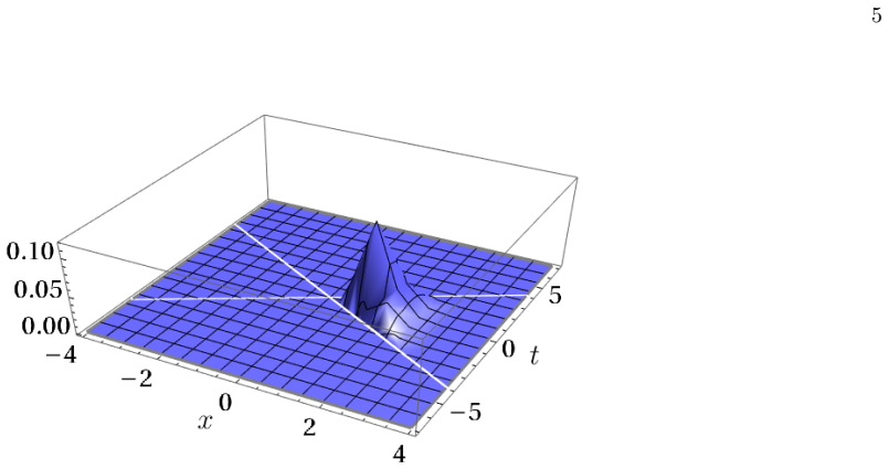


Figures from the paper (3 more)


Reference graph
Works this paper leans on
-
[1]
Second alternative: disk-supported test function 7
-
[2]
Third alternative: smooth diamond-supported test function 7
-
[3]
Conclusion 10 Acknowledgments 10 A
Fourth alternative: vertical strip-supported test function 8 V. Conclusion 10 Acknowledgments 10 A. The massive real scalar field in 1 + 1 Minkowski spacetime 10
-
[4]
Field expansion and commutation relations 10
-
[5]
Inner product and two-point functions 11
-
[6]
Physical interpretation and causality 11 References 11 I. INTRODUCTION The evaluation of entanglement entropy in relativistic Quantum Field Theory (QFT) presents a profound challenge, engaging a variety of technically demanding methods [1]. Central to the discussion of quantum information measures in Quantum Mechanics (QM) and QFT is the von Neumann entro...
work page Pith review arXiv 2025
-
[7]
Second alternative: disk-supported test function For this purpose, we choose a second test function f2(t, x) which is supported in the disk of radius a and centered at the point (b, 0), (x− b)2+ t2 ≤ a2 , (26) where the parameters (a, b) are chosen so that the disk lies within the right Rindler wedge. For the profile of the test function f2, we choose f2(...
-
[8]
Third alternative: smooth diamond-supported test function For the third type of test function, we introduce a smooth variant of the test function supported within the causal diamond ∣d+ r− x∣+ ∣t∣ ≤ r, where d denotes the center of the diamond, r is a parameter that controls its size and 8 FIG. 4. We show the behavior of the Araki-Uhlmann relative entropy...
Show all 58 references
-
[9]
It is defined as f4(t, x)= ⎧⎪⎪⎨⎪⎪⎩ e− 1 x2 −t2 e − 1 ((x2 −t2 )−β2 )((β+d)2 −(x2 −t2 )) e−(x−b)2 e−t2 , (β+ d)2 ≥ x2− t2 ≥ β2 , x ≥ ∣t∣ , 0, elsewhere
Fourth alternative: vertical strip-supported test function Finally, we introduce a fourth type of test function, which is supported in a vertical strip within the right Rindler wedge. It is defined as f4(t, x)= ⎧⎪⎪⎨⎪⎪⎩ e− 1 x2 −t2 e − 1 ((x2 −t2 )−β2 )((β+d)2 −(x2 −t2 )) e−(x−...
2025
-
[10]
The field operators satisfy the canonical commutation relations: [ak, a† q]= 2π 2ωk δ(k− q), (A2) [ak, aq]= [a† k, a† q]= 0
Field expansion and commutation relations The massive scalar field φ(x) can be expressed in terms of plane waves as: φ(x)= ∫ dk 2π 1 2ωk (e−ikµxµ ak+ eikµxµ a† k) , (A1) 11 where ωk = k0 = √ k2+ m2 is the relativistic energy dispersion relation. The field operators satisfy the...
-
[11]
These are defined as: ∆P J(f, g)= ∫ d2xd2yf(x)∆P J(x− y)g(y) , H(f, g)= ∫ d2xd2yf(x)H(x− y)g(y)
Inner product and two-point functions With the smeared fields, the Lorentz-invariant inner product between two test functions f(x) and g(x) in the vacuum state is introduced by means of the two-point smeared Wightman function ⟨f∣g⟩= ⟨0∣φ(f)φ(g)∣0⟩= i 2 ∆P J(f, g)+ H(f, g) , (A...
-
[12]
In particular, the Pauli-Jordan distri- bution, ∆ P J(x), plays a fundamental role in encoding relativistic causality, as it vanishes outside the light cone
Physical interpretation and causality Both the Hadamard and Pauli-Jordan distributions are Lorentz-invariant. In particular, the Pauli-Jordan distri- bution, ∆ P J(x), plays a fundamental role in encoding relativistic causality, as it vanishes outside the light cone. Additiona...
-
[13]
Nishioka, Rev
T. Nishioka, Rev. Mod. Phys. 90, 035007 (2018), arXiv:1801.10352 [hep-th]. 12
2018 arXiv
-
[14]
Holzhey, F
C. Holzhey, F. Larsen, and F. Wilczek, Nucl. Phys. B 424, 443 (1994), arXiv:hep-th/9403108
1994 arXiv
-
[15]
Calabrese and J
P. Calabrese and J. L. Cardy, J. Stat. Mech. 0406, P06002 (2004), arXiv:hep-th/0405152
2004 arXiv
-
[16]
Calabrese and J
P. Calabrese and J. Cardy, J. Phys. A 42, 504005 (2009), arXiv:0905.4013 [cond-mat.stat-mech]
2009 arXiv
-
[17]
Casini and M
H. Casini and M. Huerta, PoS T ASI2021, 002 (2023), arXiv:2201.13310 [hep-th]
2023 arXiv
-
[18]
Berges, S
J. Berges, S. Floerchinger, and R. Venugopalan, JHEP 04, 145, arXiv:1712.09362 [hep-th]
-
[19]
Schr¨ ofl and S
M. Schr¨ ofl and S. Floerchinger 10.1007/s00023-024-01522-2 (2023), arXiv:2307.15548 [cond-mat.stat-mech]
2023 arXiv
- [20]
- [21]
- [22]
-
[23]
Hiai and D
F. Hiai and D. Petz, Commun. Math. Phys. 143, 99 (1991)
1991
- [24]
-
[25]
D’Angelo, Class
E. D’Angelo, Class. Quant. Grav. 38, 175001 (2021), arXiv:2105.04303 [gr-qc]
2021 arXiv
-
[26]
Ciolli, R
F. Ciolli, R. Longo, A. Ranallo, and G. Ruzzi, J. Geom. Phys. 172, 104416 (2022), arXiv:2107.06787 [math-ph]
2022 arXiv
-
[27]
Galanda, A
S. Galanda, A. Much, and R. Verch, Math. Phys. Anal. Geom. 26, 21 (2023), arXiv:2305.02788 [math-ph]
2023 arXiv
-
[28]
Garbarz and G
A. Garbarz and G. Palau, Phys. Rev. D 107, 125016 (2023), arXiv:2209.00035 [hep-th]
2023 arXiv
-
[29]
Floerchinger and T
S. Floerchinger and T. Haas, Phys. Rev. E 102, 052117 (2020), arXiv:2004.13533 [cond-mat.stat-mech]
2020 arXiv
-
[30]
Dowling, S
N. Dowling, S. Floerchinger, and T. Haas, Phys. Rev. D 102, 105002 (2020), arXiv:2008.02706 [quant-ph]
2020 arXiv
-
[31]
D. L. Jafferis and S. J. Suh, JHEP 09, 068, arXiv:1412.8465 [hep-th]
-
[32]
D. L. Jafferis, A. Lewkowycz, J. Maldacena, and S. J. Suh, JHEP 06, 004, arXiv:1512.06431 [hep-th]
- [33]
-
[34]
Bousso, V
R. Bousso, V. Chandrasekaran, P. Rath, and A. Shahbazi-Moghaddam, Phys. Rev. D102, 066008 (2020), arXiv:2007.00230 [hep-th]
2020 arXiv
-
[35]
Tomita, Fifth Functional Analysis Sympos (Tˆ ohoku Univ., Sendai, 1967), Math
M. Tomita, Fifth Functional Analysis Sympos (Tˆ ohoku Univ., Sendai, 1967), Math. Inst., Tohoku Univ., Sendai , 101 (1967)
1967
-
[36]
Takesaki, Tomita’s Theory of Modular Hilbert Algebras and its Applications , Lecture Notes in Mathematics (Springer- Verlag, 1970)
M. Takesaki, Tomita’s Theory of Modular Hilbert Algebras and its Applications , Lecture Notes in Mathematics (Springer- Verlag, 1970)
1970
-
[37]
Araki, Publ
H. Araki, Publ. Res. Inst. Math. Sci. Kyoto 1976, 809 (1976)
1976
-
[38]
Uhlmann, Commun
A. Uhlmann, Commun. Math. Phys. 54, 21 (1977)
1977
- [39]
-
[40]
Casini, E
H. Casini, E. Teste, and G. Torroba, J. Phys. A 50, 364001 (2017), arXiv:1703.10656 [hep-th]
2017 arXiv
-
[41]
Hollands and A
S. Hollands and A. Ishibashi, Class. Quant. Grav. 36, 195001 (2019), arXiv:1904.00007 [gr-qc]
2019 arXiv
-
[42]
Casini, S
H. Casini, S. Grillo, and D. Pontello, Phys. Rev. D 99, 125020 (2019), arXiv:1903.00109 [hep-th]
2019 arXiv
- [43]
-
[44]
Morinelli, Y
V. Morinelli, Y. Tanimoto, and B. Wegener, Commun. Math. Phys. 395, 331 (2022), arXiv:2107.00039 [math-ph]
2022 arXiv
-
[45]
Casini, I
H. Casini, I. Salazar Landea, and G. Torroba, Phys. Rev. Lett. 130, 111603 (2023), arXiv:2212.10575 [hep-th]
2023 arXiv
-
[46]
D’Angelo, M
E. D’Angelo, M. B. Fr¨ ob, S. Galanda, P. Meda, A. Much, and K. Papadopoulos, PTEP 2024, 021A01 (2024), arXiv:2311.13990 [hep-th]
2024 arXiv
-
[47]
M. B. Fr¨ ob, A. Much, and K. Papadopoulos, Phys. Rev. D 108, 105004 (2023), arXiv:2310.12185 [gr-qc]
2023 arXiv
-
[48]
Katsinis and G
D. Katsinis and G. Pastras, Phys. Rev. D 110, 085015 (2024), arXiv:2406.11031 [hep-th]
2024 arXiv
-
[49]
Abate and G
N. Abate and G. Torroba, SciPost Phys. 18, 029 (2025), arXiv:2409.18186 [hep-th]
2025 arXiv
- [50]
-
[51]
Ciolli, R
F. Ciolli, R. Longo, and G. Ruzzi, Commun. Math. Phys. 379, 979 (2019), arXiv:1906.01707 [math-ph]
2019 arXiv
-
[52]
M. B. Fr¨ ob and L. Sangaletti, (2024), arXiv:2411.09696 [math-ph]
2024 arXiv
-
[53]
J. J. Bisognano and E. H. Wichmann, J. Math. Phys. 16, 985 (1975)
1975
-
[54]
M. S. Guimaraes, I. Roditi, and S. P. Sorella, (2024), arXiv:2411.03485 [quant-ph]
2024 arXiv
-
[55]
M. S. Guimaraes, I. Roditi, S. P. Sorella, and A. F. Vieira, (2025), arXiv:2501.03186 [quant-ph]
2025 arXiv
-
[56]
Coleman, Physical Review D 11, 2088 (1975)
S. Coleman, Physical Review D 11, 2088 (1975)
1975
-
[57]
Gomez Nicola and D
A. Gomez Nicola and D. A. Steer, Nucl. Phys. B 549, 409 (1999), arXiv:hep-ph/9810519
1999 arXiv
-
[58]
Haag, Local quantum physics: Fields, particles, algebras (1992)
R. Haag, Local quantum physics: Fields, particles, algebras (1992)
1992
Reviewed August 7, 2026 · model on record in the stance chip above.
Discussion (0). Continue with ORCID to comment.