REVIEW 6 minor 114 references
Flickers, Bursts, and Dips: Detecting Rapid Variability with the g(2) Autocorrelation Function
T0 review · 0 major / 6 minor · reviewed 2026-08-16 · deepseek-v4-flash
Pith's one-line read The paper argues that the normalized autocorrelation function g(2) of ordinary photometry can expose chaotic, nonperiodic variability on sub-millisecond timescales, even when each individual fluctuation is far too weak to detect on its own.
desk verdict A careful, useful methods paper on using g(2) for sub-millisecond chaotic variability; the estimator and variance derivations are sound, but the PANOSETI sensitivity claim in §3.1.1 is off by orders of magnitude and needs fixing. read the letter →
The pith
A machine-rendered reading of the paper's core claim, the machinery that carries it, and where it could break.
The reading
What carries the argument
The key object is the normalized intensity autocorrelation $g^{(2)}(\Delta t)=\langle I(t)I(t+\Delta t)\rangle/\langle I(t)\rangle^2$ for a stationary light curve; its excess over 1 equals the variance of fractional intensity fluctuations, and a compact bump at short lags marks variability with coherence time $\tau_c$. The load-bearing estimator is $\Delta\hat{g}^{(2)}(\Delta i, \Delta j)$, formed from products $(Q_i-Q_{i+\Delta i+\Delta j})(Q_{i+\Delta i}-Q_{i+\Delta j})$ normalized by the mean count squared; it estimates $g^{(2)}(\Delta i\,T_d)-g^{(2)}(\Delta j\,T_d)$ while suppressing shot noise at zero lag and linear-in-fluctuation residuals. Gaussian-process covariance calculations using Isserlis's theorem, together with Poisson shot-noise moment calculations, give the variance of this estimator, from which the signal-to-noise ratio and the required number of data points follow.
What would settle it
Record an hour of continuous microsecond-cadence photometry of a bright, apparently constant star with a fast photon-counting camera, compute $\Delta\hat{g}^{(2)}(1, \Delta j)$, and compare the scatter to the shot-noise variance formula $(2+\delta_{0,\Delta i})/(N \bar{I}_d^2)$; a bump or excess scatter not predicted by the formula would falsify the estimator's variance model, while flat results at the predicted noise level would support the method.
Extended reading notes
Core claim
The central claim is that any new, chaotic source of variability imprints an extra bump on $g^{(2)}(t)$ centered at zero lag with width set by the variability's coherence time $\tau_c$, and that the height of this bump can be isolated with the difference estimator $\Delta\hat{g}^{(2)}(\Delta i, \Delta j)$, which compares photon products at two lags and removes both the zero-lag shot-noise spike and residual terms linear in the fluctuations. The signal is quadratic in intensity: when the variable source is blended into a brighter background, the bump height is diluted by the square of the flux ratio. The paper shows that shot noise and scintillation limit the measurement in calculable ways, and that with enough data a bump is detectable even when each individual fluctuation event has signal-to-noise around one. Three model applications -- a flickering artificial lantern beside a star, optical microbursts from the Crab pulsar, and frequent shallow cometary transits -- are simulated to demonstrate that the predicted sensitivity is real.
Load-bearing premise
The method assumes the rapid-variability signal is an additive, independent, zero-mean fluctuation on a constant background, and that slower background variability such as atmospheric scintillation is either much longer in coherence time or removable by comparison with a control star.
Editorial extensions
If this is right
- Sub-millisecond chaotic variability from sources like the Crab pulsar can be detected in about an hour of IACT photometry even when the microbursts have signal-to-noise near one individually.
- A quasithermal lantern with mean flux about $10^{-3}$ of its host star is detectable around an 8th-magnitude sunlike star within about a minute of observation.
- Frequent shallow cometary transits that are too weak to detect individually will appear as a bump in $g^{(2)}$ of TESS-like light curves.
- Because the signal is quadratic in the source-to-background flux ratio, blended backgrounds suppress it quadratically; the most promising targets are bright stars observed with large collecting areas.
- The variance formulas give a scaling law for the required number of data points, roughly $N_d \propto (\text{noise}/\text{variability})^4$, which quantifies when the autocorrelation method beats direct event detection.
Reading between the lines
- The same $\Delta\hat{g}^{(2)}$ estimator could be applied to archival continuous light curves from missions like TESS to search for irregular transit swarms, an extension beyond the three worked models.
- A differential mode comparing $\Delta\hat{g}^{(2)}$ on target and control sightlines could suppress ubiquitous terrestrial backgrounds such as unexcised Cherenkov showers; the paper suggests this but does not develop it fully.
- Real detectors with dead time or non-Poisson noise, such as silicon photomultipliers, would require revised variance formulas; the paper notes the factor-of-two noise penalty for one common SiPM model, so the sensitivity numbers are a best case.
- If optical SETI instruments switch from triggered to continuous recording modes, $g^{(2)}$ analysis could convert existing pulse-hunting hardware into statistical variability searches without storing the full light curves.
Signed reviews
Editorial analysis
A structured set of objections, weighed in public.
Referee Report
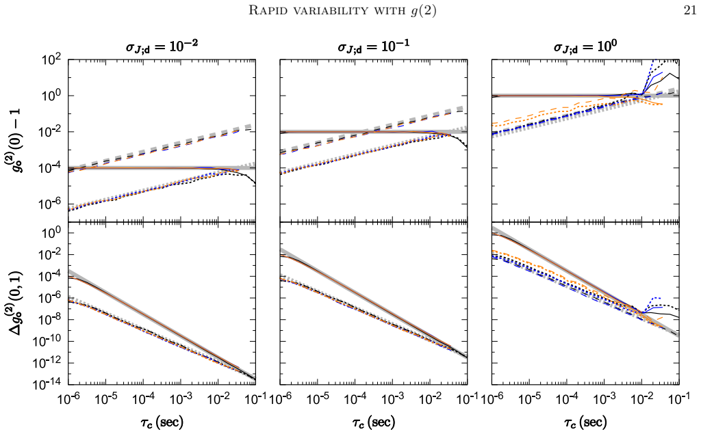
Summary. The paper proposes using the normalized autocorrelation function g(2) to detect fast, chaotic optical variability whose individual fluctuations are buried in shot noise and scintillation. It introduces a differenced estimator Δĝ(2), derives its mean and variance for Gaussian variability and for shot noise in Appendices A and B, and derives signal-to-noise scalings in Section 2.9. Three applications are presented: a modulated 'quasithermal lantern' near a host star observed with an IACT-like array, optical microbursts in the Crab pulsar, and irregular cometary transits in TESS-like photometry. The central claim is that fluctuations with individual signal-to-noise S_Q ≈ 1 can be detected statistically once enough independent samples are accumulated. I checked the specific stress-test concern about Eqs. (37) and (39): inserting the stated lantern parameters into Eq. (37) gives S_g2 ≈ 3.1, and inserting the PANOSETI parameters into Eq. (39) gives S_g2 ≈ 75 for a 1000 h integration at J = 10^-3, in agreement with Eq. (32) to within factors of order unity; the alleged six-order-of-magnitude discrepancy does not reproduce. The main derivations are internally consistent, and the simulations in Figure 4 support the analytic variance scalings.
Significance. If the result holds, the method provides a broadly applicable statistical tool for sub-millisecond optical variability, complementing individual-pulse searches and periodicity folding. The paper's strengths are its first-principles derivations in Appendices A and B, explicit analytic SNR scalings, and numerical simulations that verify the variance formulas. The three worked examples give concrete, falsifiable predictions about how many data points are needed to detect S_Q ≈ 1 fluctuations. The connection to earlier MANIA d2 work and stellar-variability autocorrelation studies is acknowledged, so the novelty claim is appropriately scoped as a synthesis and quantitative generalization rather than a claim of a wholly new statistic. The paper is not circular: the SNR formulas are derived, and the simulations generate light curves from assumed covariances and verify that the estimator recovers those covariances.
minor comments (6)
- [Section 2.9, Eq. (31)] The standard-deviation formula as printed has N_d^o in the denominator without a square root; this contradicts the shot-noise variance in Appendix B, Eq. (B30), and makes Eq. (32) not derivable from Eq. (31). The denominator should be sqrt(N_d^o).
- [Section 2.9, Eqs. (33) and (36)] Eq. (33) contains an extra factor of η^2 beyond what Eq. (32) implies: solving Eq. (32) for N_d^o gives a factor 2η^4, not 2η^2(...)^4 = 2η^6. Similarly, Eq. (36) omits the S_Q^4 factor that follows from Eq. (35). The numerical examples use S_Q ≈ 1 and η ≈ 1, so the conclusions are unaffected, but the general formulas should be corrected.
- [Section 3.1.1 and footnote 9] The lantern model assumes 1 μs continuous sampling and a 10 μs coherence time, but footnote 9 states that VERITAS has a reported maximum sampling rate of 4.8 kHz. Please state explicitly that the example assumes a hypothetical upgraded continuous-readout mode, or rescale the example to T_d ≈ 208 μs, in which case the quoted sensitivity changes substantially.
- [Section 3.3] The transit example describes a habitable-zone transit timescale of about 3 hr, but for a solar-radius star at 1 au with v_T = 30 km/s the full transit duration is approximately 13 hr. Clarify the assumed stellar radius and orbital parameters.
- [Figure 4 caption and general typography] The caption writes '2 16 samples' where 2^16 is intended; please fix this and scan the equations for similar missing exponents or square-root symbols.
- [Sections 2.1 and 2.8] The paper states the assumption of no dead time in Section 2.1 but does not revisit it in the variance formulas. A sentence noting that dead time, correlated detector noise, or target-correlated scintillation would require revised variance expressions would help readers apply the method to real instruments.
Circularity Check
No significant circularity: the SNR formulas are derived from first principles, and the simulations are self-consistency checks rather than fitted predictions.
full rationale
The derivation chain is self-contained. The Delta-g(2) estimator is defined directly from the photon-count time series (Eq. 9), and its mean and variance are obtained from the Poisson shot-noise model (Appendix B) and from a multivariate-normal Gaussian-variability model (Appendix A) using Isserlis' theorem; no parameter is fitted to the simulations. The Sg2 formula (Eq. 32) follows algebraically from those variances, and the example sensitivity estimates (Eqs. 37 and 39) are evaluations of that formula for stated instrument parameters. The simulations inject light curves with an assumed covariance and then verify that the estimator recovers that covariance; this is an internal self-consistency check, which is appropriate for a methods paper, and it does not make a prediction equivalent to its input by construction. The two self-citations (Lacki 2011 and Lacki 2024) support peripheral facts about IACT collecting area and Poisson-process background, with external support such as Kingman (1993) also cited, so they are not load-bearing. The paper's stated limitations (scintillation confusion, Durbin-Watson degeneracy, neglected dead time) concern robustness and correctness rather than circularity; the apparent numerical mismatch between Eq. 32 and the printed prefactors in Eqs. 37/39 is an internal consistency issue, not a reduction of a claim to its inputs. No circular step is therefore established.
Assumptions & free parameters
free parameters (9)
- Lantern fractional brightness relative to host star =
10^-3, 10^-3.5, and 10^-2.75 in the examples
- Host star V magnitude in the lantern example =
V = 8
- Photon detection efficiency of the VERITAS-like array =
15%
- Lantern coherence time and sampling cadence =
tau_c = 10 microseconds; T_d = 1 microsecond
- Crab microburst peak intensity =
Set so S_Q is near 1
- Crab microburst width and sampling cadence =
0.5 microsecond FWHM; T_d = 0.1 microsecond
- Crab nebula background photon flux =
7e6 photon m^-2 s^-1
- Comet transit depth and event rate =
Varied in Figure 3
- TESS-like star magnitude and binned cadence =
IC = 12; T_d = 3 hours after binning
assumptions (8)
- domain assumption The photometric intensity is wide-sense stationary or cyclostationary, so the autocorrelation depends only on lag.
- domain assumption Independent variability mechanisms add linearly in flux and in covariance.
- domain assumption Photon counts are Poisson distributed given the intensity.
- domain assumption Atmospheric scintillation can be modeled as stationary Gaussian noise with a broken power-law spectrum, with lognormal corrections simulated separately.
- ad hoc to paper The intrinsic autocovariance has a Gaussian shape for the analytic variance estimates.
- standard math Isserlis' theorem for zero-mean multivariate normal variables is applied to compute moments of intensity products.
- standard math Campbell's theorem for Poisson point processes gives the mean and covariance of burst and transit intensities.
- domain assumption The observing series is uninterrupted with no dead time.
invented entities (1)
-
Quasithermal lantern, an artificial modulated beacon near a host star
Cite this review
Pith. "Pith review of Flickers, Bursts, and Dips: Detecting Rapid Variability with the g(2) Autocorrelation Function." pith.science (2026). https://pith.science/paper/U7BWKN57
@misc{pith2026250421157,
  author       = {Pith},
  title        = {Pith review of: Flickers, Bursts, and Dips: Detecting Rapid Variability with the g(2) Autocorrelation Function},
  year         = {2026},
  howpublished = {\url{https://pith.science/paper/U7BWKN57}},
  note         = {Machine review of arXiv:2504.21157}
}
abstract
Rapid optical transient events can be hard to detect because of the limited number of photons they produce. I discuss a method of inferring the presence of fast, chaotic variability in photometry using the normalized autocorrelation function, what is called $g^{(2)}$ in quantum optics. The variability's signature is a bump in the function at short lags. No periodicity is needed for the method to work. Versions of this method are attested in stellar variability studies, but its uses in some other subfields apparently have not been realized. I calculate expected signal-to-noise ratios with shot noise and scintillation. This method could be used to find unknown phenomena, particularly sub-millisecond optical variability. I present simple models of three example use cases: a flickering artificial "lantern" near a host sun, optical microbursts from the Crab pulsar, and frequent irregular transits of a star by cometary bodies.
Figures


Figures from the paper (1 more)
Reference graph
Works this paper leans on
-
[1]
2016, PhRvL, 117, 111301, doi: 10.1103/PhysRevLett.117.111301
Abdallah, H., Abramowski, A., Aharonian, F., et al. 2016, PhRvL, 117, 111301, doi: 10.1103/PhysRevLett.117.111301
-
[2]
Abe, S., Abhir, J., Acciari, V. A., et al. 2024, MNRAS, 529, 4387, doi: 10.1093/mnras/stae697
-
[3]
U., Archambault, S., Archer, A., et al
Abeysekara, A. U., Archambault, S., Archer, A., et al. 2016, ApJL, 818, L33, doi: 10.3847/2041-8205/818/2/L33
-
[4]
U., Benbow, W., Brill, A., et al
Abeysekara, A. U., Benbow, W., Brill, A., et al. 2020, Nature Astronomy, 4, 1164, doi: 10.1038/s41550-020-1143-y
-
[5]
2012, ApJ, 757, 158, doi: 10.1088/0004-637X/757/2/158
Abramowski, A., Acero, F., Aharonian, F., et al. 2012, ApJ, 757, 158, doi: 10.1088/0004-637X/757/2/158
-
[6]
Acharyya, A., Adams, C. B., Archer, A., et al. 2023, AJ, 166, 84, doi: 10.3847/1538-3881/ace347
-
[7]
Acharyya, A., Aufdenberg, J. P., Bangale, P., et al. 2024, ApJ, 966, 28, doi: 10.3847/1538-4357/ad2b68
-
[8]
Actis, M., Agnetta, G., Aharonian, F., et al. 2011, Experimental Astronomy, 32, 193, doi: 10.1007/s10686-011-9247-0 Aleksi´ c, J., Ansoldi, S., Antonelli, L. A., et al. 2014, JCAP, 2014, 008, doi: 10.1088/1475-7516/2014/02/008
Show all 114 references
-
[9]
2017, Nature Astronomy, 1, 854, doi: 10.1038/s41550-017-0266-2
Ambrosino, F., Papitto, A., Stella, L., et al. 2017, Nature Astronomy, 1, 854, doi: 10.1038/s41550-017-0266-2
2017 doi
-
[10]
A., et al
Ansdell, M., Gaidos, E., Rappaport, S. A., et al. 2016, ApJ, 816, 69, doi: 10.3847/0004-637X/816/2/69
2016 doi
-
[11]
L., et al
Ansdell, M., Gaidos, E., Jacobs, T. L., et al. 2019, MNRAS, 483, 3579, doi: 10.1093/mnras/sty3289
2019 doi
-
[12]
A., Antoranz, P., et al
Ansoldi, S., Antonelli, L. A., Antoranz, P., et al. 2016, A&A, 585, A133, doi: 10.1051/0004-6361/201526853
2016 doi
-
[13]
Arecchi, F. T. 1965, PhRvL, 15, 912, doi: 10.1103/PhysRevLett.15.912
1965 doi
-
[14]
Arnold, L. F. A. 2005, ApJ, 627, 534, doi: 10.1086/430437
2005 doi
-
[15]
A., Davoyan, A
Atwater, H. A., Davoyan, A. R., Ilic, O., et al. 2018, Nature Materials, 17, 861, doi: 10.1038/s41563-018-0075-8
2018 doi
-
[16]
2007, in Stochastic Geometry, ed
Baddeley, A. 2007, in Stochastic Geometry, ed. W. Weil (Berlin: Springer), 1–75, doi: 10.1007/978-3-540-38175-4 1
2007 doi
-
[17]
2009, Journal of Modern Optics, 56, 261, doi: 10.1080/09500340802450565
Barbieri, C., Naletto, G., Occhipinti, T., et al. 2009, Journal of Modern Optics, 56, 261, doi: 10.1080/09500340802450565
2009 doi
-
[18]
A., Stassun, K
Bastien, F. A., Stassun, K. G., Basri, G., & Pepper, J. 2013, Nature, 500, 427, doi: 10.1038/nature12419
2013 doi
-
[19]
2019, Nature Astronomy, 3, 511, doi: 10.1038/s41550-019-0741-z
Benbow, W., Bird, R., Brill, A., et al. 2019, Nature Astronomy, 3, 511, doi: 10.1038/s41550-019-0741-z
2019 doi
-
[20]
1997, Ap&SS, 252, 51, doi: 10.1023/A:1000845628229 24 Lacki
Beskin, G., Borisov, N., Komarova, V., et al. 1997, Ap&SS, 252, 51, doi: 10.1023/A:1000845628229 24 Lacki
1997 doi
-
[21]
L., & Shvartsman, V
Plakhotnichenko, V. L., & Shvartsman, V. F. 1982, in Astrophysics and Space Science Library, Vol. 92, IAU Colloq. 67: Instrumentation for Astronomy with Large Optical Telescopes, ed. C. M. Humphries, 181–184, doi: 10.1007/978-94-009-7787-7 23
1982 doi
-
[22]
M., Mitronova, S
Beskin, G. M., Mitronova, S. N., Neizvestny, S. I., et al. 1995, Astronomical and Astrophysical Transactions, 8, 297, doi: 10.1080/10556799508226946
1995 doi
-
[23]
Bodman, E. H. L., & Quillen, A. 2016, ApJL, 819, L34, doi: 10.3847/2041-8205/819/2/L34
2016 doi
-
[24]
Borra, E. F. 2010, A&A, 511, L6, doi: 10.1051/0004-6361/200913878 —. 2012, AJ, 144, 181, doi: 10.1088/0004-6256/144/6/181
2010 doi
-
[25]
F., & Trottier, E
Borra, E. F., & Trottier, E. 2016, PASP, 128, 114201, doi: 10.1088/1538-3873/128/969/114201
2016 doi
-
[26]
S., LaCourse, D
Boyajian, T. S., LaCourse, D. M., Rappaport, S. A., et al. 2016, MNRAS, 457, 3988, doi: 10.1093/mnras/stw218
2016 doi
-
[27]
S., Alonso, R., Ammerman, A., et al
Boyajian, T. S., Alonso, R., Ammerman, A., et al. 2018, ApJL, 853, L8, doi: 10.3847/2041-8213/aaa405
2018 doi
-
[28]
Brzycki, B., Siemion, A. P. V., de Pater, I., et al. 2023, ApJ, 952, 46, doi: 10.3847/1538-4357/acdee0
2023 doi
-
[29]
M., & Drummond, P
Caves, C. M., & Drummond, P. D. 1994, Reviews of Modern Physics, 66, 481, doi: 10.1103/RevModPhys.66.481
1994 doi
-
[30]
2019, The Analysis of Time Series: An Introduction with R (Boca Raton: Chapman and Hall/CRC)
Chatfield, C., & Xing, H. 2019, The Analysis of Time Series: An Introduction with R (Boca Raton: Chapman and Hall/CRC)
2019
-
[31]
N., Stoyan, D., Kendall, W
Chiu, S. N., Stoyan, D., Kendall, W. S., & Mecke, J. 2013, Stochastic Geometry and its Applications: Third Edition (New York: Wiley), doi: 10.1002/9781118658222
2013 doi
-
[32]
J., Disney, M
Cocke, W. J., Disney, M. J., & Taylor, D. J. 1969, Nature, 221, 525, doi: 10.1038/221525a0
1969 doi
-
[33]
M., & Hillenbrand, L
Cody, A. M., & Hillenbrand, L. A. 2010, ApJS, 191, 389, doi: 10.1088/0067-0049/191/2/389
2010 doi
-
[34]
M., Soto, A
Corbett, H., Law, N. M., Soto, A. V., et al. 2020, ApJL, 903, L27, doi: 10.3847/2041-8213/abbee5
2020 doi
-
[35]
M., Lazio, J
Cordes, J. M., Lazio, J. W., & Sagan, C. 1997, ApJ, 487, 782, doi: 10.1086/304620
1997 doi
-
[36]
2009, Astroparticle Physics, 31, 156, doi: 10.1016/j.astropartphys.2008.12.008
Deil, C., Domainko, W., Hermann, G., et al. 2009, Astroparticle Physics, 31, 156, doi: 10.1016/j.astropartphys.2008.12.008
2009 doi
-
[37]
S., Marsh, T
Dhillon, V. S., Marsh, T. R., Stevenson, M. J., et al. 2007, MNRAS, 378, 825, doi: 10.1111/j.1365-2966.2007.11881.x
2007
-
[39]
S., Bezawada, N., Black, M., et al
Dhillon, V. S., Bezawada, N., Black, M., et al. 2021, MNRAS, 507, 350, doi: 10.1093/mnras/stab2130
2021 doi
-
[40]
J., & Milone, A
Dobrzycka, D., Kenyon, S. J., & Milone, A. A. E. 1996, AJ, 111, 414, doi: 10.1086/117794
1996 doi
-
[41]
1994, The Messenger, 78, 9
Dravins, D. 1994, The Messenger, 78, 9
1994
-
[42]
Dravins, D., Lindegren, L., Mezey, E., & Young, A. T. 1997, PASP, 109, 173, doi: 10.1086/133872 —. 1998, PASP, 110, 610, doi: 10.1086/316161
1997 doi
- [43]
-
[44]
Durbin, J., & Watson, G. S. 1950, Biometrika, 37, 409, doi: 10.2307/2332391 —. 1951, Biometrika, 38, 159, doi: 10.2307/2332325
1950 doi
-
[45]
2000, PhRvL, 85, 2669, doi: 10.1103/PhysRevLett.85.2669
Eichler, D., & Beskin, G. 2000, PhRvL, 85, 2669, doi: 10.1103/PhysRevLett.85.2669
2000 doi
-
[46]
M., & Uttley, P
Emmanoulopoulos, D., McHardy, I. M., & Uttley, P. 2010, MNRAS, 404, 931, doi: 10.1111/j.1365-2966.2010.16328.x
2010
-
[47]
2018, MNRAS, 478, 1209, doi: 10.1093/mnras/sty1122
Farah, W., Flynn, C., Bailes, M., et al. 2018, MNRAS, 478, 1209, doi: 10.1093/mnras/sty1122
2018 doi
-
[48]
M., & Vidal-Madjar, A
Ferlet, R., Hobbs, L. M., & Vidal-Madjar, A. 1987, A&A, 185, 267
1987
-
[49]
2013, ApJ, 768, 93, doi: 10.1088/0004-637X/768/1/93
Findeisen, K., Hillenbrand, L., Ofek, E., et al. 2013, ApJ, 768, 93, doi: 10.1088/0004-637X/768/1/93
2013 doi
-
[50]
2009, A&A, 507, 1719, doi: 10.1051/0004-6361/200911739 German` a, C., Zampieri, L., Barbieri, C., et al
Foellmi, C. 2009, A&A, 507, 1719, doi: 10.1051/0004-6361/200911739 German` a, C., Zampieri, L., Barbieri, C., et al. 2012, A&A, 548, A47, doi: 10.1051/0004-6361/201118754
2009 doi
-
[51]
2017, MNRAS, 472, 4126, doi: 10.1093/mnras/stx2143 H
Guerin, W., Dussaux, A., Fouch´ e, M., et al. 2017, MNRAS, 472, 4126, doi: 10.1093/mnras/stx2143 H. E. S. S. Collaboration, Aharonian, F., Ait Benkhali, F., et al. 2022, A&A, 662, A65, doi: 10.1051/0004-6361/202243096
2017 doi
-
[52]
2013, Stochastic Geometry for Wireless Networks (Cambridge: Cambridge University Press), doi: 10.1017/cbo9781139043816 Hanbury Brown, R
Haenggi, M. 2013, Stochastic Geometry for Wireless Networks (Cambridge: Cambridge University Press), doi: 10.1017/cbo9781139043816 Hanbury Brown, R. 1956a, Nature, 178, 1447, doi: 10.1038/1781447a0 —. 1956b, Nature, 178, 1046, doi: 10.1038/1781046a0 Hanbury Brown, R., Davis, J...
2013 doi
- [53]
-
[54]
H., Jones, G., & Eilek, J
Hankins, T. H., Jones, G., & Eilek, J. A. 2015, ApJ, 802, 130, doi: 10.1088/0004-637X/802/2/130
2015 doi
-
[55]
H., Kern, J
Hankins, T. H., Kern, J. S., Weatherall, J. C., & Eilek, J. A. 2003, Nature, 422, 141, doi: 10.1038/nature01477
2003 doi
-
[56]
K., Dhillon, V
Hardy, L. K., Dhillon, V. S., Spitler, L. G., et al. 2017, MNRAS, 472, 2800, doi: 10.1093/mnras/stx2153
2017 doi
-
[57]
R., Ackermann, R
Harp, G. R., Ackermann, R. F., Astorga, A., et al. 2018, ApJ, 869, 66, doi: 10.3847/1538-4357/aaeb98 Rapid variability with g(2) 25
2018 doi
-
[58]
E., Farley, O
Hartley, K. E., Farley, O. J. D., Townson, M. J., Osborn, J., & Wilson, R. W. 2023, MNRAS, 526, 1235, doi: 10.1093/mnras/stad2835
2023 doi
- [59]
-
[60]
2006, Astroparticle Physics, 26, 22, doi: 10.1016/j.astropartphys.2006.04.008
Hinton, J., Hermann, G., Kr¨ otz, P., & Funk, S. 2006, Astroparticle Physics, 26, 22, doi: 10.1016/j.astropartphys.2006.04.008
2006 doi
-
[61]
2019, PASP, 131, 034502, doi: 10.1088/1538-3873/aafbac —
Hippke, M. 2019, PASP, 131, 034502, doi: 10.1088/1538-3873/aafbac —. 2021, AJ, 162, 1, doi: 10.3847/1538-3881/abf7b7
2019 doi
-
[62]
B., & Horowitz, P
Howard, A. B., & Horowitz, P. 2001, in Society of Photo-Optical Instrumentation Engineers (SPIE) Conference Series, Vol. 4273, The Search for Extraterrestrial Intelligence (SETI) in the Optical Spectrum III, ed. S. A. Kingsley & R. Bhathal, 153–160, doi: 10.1117/12.435369
2001 doi
-
[63]
W., Horowitz, P., Wilkinson, D
Howard, A. W., Horowitz, P., Wilkinson, D. T., et al. 2004, ApJ, 613, 1270, doi: 10.1086/423300
2004 doi
-
[64]
Isaacson, H., Siemion, A. P. V., Marcy, G. W., et al. 2019, PASP, 131, 014201, doi: 10.1088/1538-3873/aaeae0
2019 doi
-
[65]
1918, Biometrika, 12, 134, doi: 10.2307/2331932
Isserlis, L. 1918, Biometrika, 12, 134, doi: 10.2307/2331932
1918 doi
-
[66]
2014, A&A, 570, A41, doi: 10.1051/0004-6361/201424313
Kallinger, T., De Ridder, J., Hekker, S., et al. 2014, A&A, 570, A41, doi: 10.1051/0004-6361/201424313
2014 doi
-
[67]
Kingman, J. F. C. 1993, Poisson Processes (Oxford: Clarendon Press), doi: 10.1093/oso/9780198536932.001.0001
1993
-
[68]
2019, Research Notes of the American Astronomical Society, 3, 91, doi: 10.3847/2515-5172/ab2fdb
Kipping, D. 2019, Research Notes of the American Astronomical Society, 3, 91, doi: 10.3847/2515-5172/ab2fdb
2019 doi
-
[69]
2012, MNRAS, 426, 647, doi: 10.1111/j.1365-2966.2012.21653.x
Kornilov, V. 2012, MNRAS, 426, 647, doi: 10.1111/j.1365-2966.2012.21653.x
2012
-
[70]
2012, A&A, 546, A41, doi: 10.1051/0004-6361/201219954 Kov´ acs, G., Zucker, S., & Mazeh, T
Voziakova, O. 2012, A&A, 546, A41, doi: 10.1051/0004-6361/201219954 Kov´ acs, G., Zucker, S., & Mazeh, T. 2002, A&A, 391, 369, doi: 10.1051/0004-6361:20020802
2012 doi
-
[71]
Lacki, B. C. 2011, MNRAS, 416, 3075, doi: 10.1111/j.1365-2966.2011.19255.x —. 2024, ApJ, 966, 182, doi: 10.3847/1538-4357/ad11f2 Le Bohec, S., & Holder, J. 2006, ApJ, 649, 399, doi: 10.1086/506379
2011
-
[72]
R., Poppe, A., Hammel, E., et al
Leeb, W. R., Poppe, A., Hammel, E., et al. 2013, Astrobiology, 13, 521, doi: 10.1089/ast.2012.0951
2013
- [73]
-
[74]
A., Antoranz, P., et al
Lucarelli, F., Barrio, J. A., Antoranz, P., et al. 2008, Nuclear Instruments and Methods in Physics Research A, 589, 415, doi: 10.1016/j.nima.2008.03.007
2008 doi
-
[75]
A., Werthimer, D., et al
Maire, J., Wright, S. A., Werthimer, D., et al. 2020, in Society of Photo-Optical Instrumentation Engineers (SPIE) Conference Series, Vol. 11454, X-Ray, Optical, and Infrared Detectors for Astronomy IX, ed. A. D. Holland & J. Beletic, 114543C, doi: 10.1117/12.2562786
2020 doi
-
[76]
1964, American Journal of Physics, 32, 919, doi: 10.1119/1.1970023
Martienssen, W., & Spiller, E. 1964, American Journal of Physics, 32, 919, doi: 10.1119/1.1970023
1964 doi
-
[77]
2011, ApJ, 741, 119, doi: 10.1088/0004-637X/741/2/119
Mathur, S., Hekker, S., Trampedach, R., et al. 2011, ApJ, 741, 119, doi: 10.1088/0004-637X/741/2/119
2011 doi
-
[78]
P., Mannings, V., & Ungerechts, H
Natta, A., Grinin, V. P., Mannings, V., & Ungerechts, H. 1997, ApJ, 491, 885, doi: 10.1086/305006
1997 doi
-
[79]
Nimmo, K., Hessels, J. W. T., Keimpema, A., et al. 2021, Nature Astronomy, 5, 594, doi: 10.1038/s41550-021-01321-3
2021 doi
-
[80]
S., & Wilson, R
Osborn, J., F¨ ohring, D., Dhillon, V. S., & Wilson, R. W. 2015, MNRAS, 452, 1707, doi: 10.1093/mnras/stv1400 Preuß, S., Hermann, G., Hofmann, W., & Kohnle, A. 2002, Nuclear Instruments and Methods in Physics Research A, 481, 229, doi: 10.1016/S0168-9002(01)01264-5
2015 doi
-
[81]
1999, in Astronomical Society of the Pacific Conference Series, Vol
Radhakrishnan, V. 1999, in Astronomical Society of the Pacific Conference Series, Vol. 180, Synthesis Imaging in Radio Astronomy II, ed. G. B. Taylor, C. L. Carilli, & R. A. Perley, 671
1999
-
[82]
2012, ApJ, 752, 1, doi: 10.1088/0004-637X/752/1/1
Rappaport, S., Levine, A., Chiang, E., et al. 2012, ApJ, 752, 1, doi: 10.1088/0004-637X/752/1/1
2012 doi
-
[83]
2018, MNRAS, 474, 1453, doi: 10.1093/mnras/stx2735
Rappaport, S., Vanderburg, A., Jacobs, T., et al. 2018, MNRAS, 474, 1453, doi: 10.1093/mnras/stx2735
2018 doi
-
[84]
2020, A&A, 639, A11, doi: 10.1051/0004-6361/201936071
Rebollido, I., Eiroa, C., Montesinos, B., et al. 2020, A&A, 639, A11, doi: 10.1051/0004-6361/201936071
2020 doi
-
[85]
Reiger, S. H. 1963, AJ, 68, 395, doi: 10.1086/108990
1963 doi
-
[86]
R., Winn, J
Ricker, G. R., Winn, J. N., Vanderspek, R., et al. 2014, in Society of Photo-Optical Instrumentation Engineers (SPIE) Conference Series, Vol. 9143, Space Telescopes and Instrumentation 2014: Optical, Infrared, and Millimeter Wave, ed. J. Oschmann, Jacobus M., M. Clampin, G. G....
2014 doi
-
[87]
2015, ApJ, 812, 112, doi: 10.1088/0004-637X/812/2/112
Sanchis-Ojeda, R., Rappaport, S., Pall` e, E., et al. 2015, ApJ, 812, 112, doi: 10.1088/0004-637X/812/2/112
2015 doi
-
[88]
J., Kording, E., et al
Scaringi, S., Maccarone, T. J., Kording, E., et al. 2015, Science Advances, 1, e1500686, doi: 10.1126/sciadv.1500686
2015 doi
-
[89]
E., Pedersen, H., Gouiffes, C., Poulsen, J
Schaefer, B. E., Pedersen, H., Gouiffes, C., Poulsen, J. M., & Pizzichini, G. 1987, A&A, 174, 338
1987
-
[90]
N., & Townes, C
Schwartz, R. N., & Townes, C. H. 1961, Nature, 190, 205, doi: 10.1038/190205a0
1961 doi
-
[91]
2003, Science, 301, 493, doi: 10.1126/science.1084919 26 Lacki
Shearer, A., Stappers, B., O’Connor, P., et al. 2003, Science, 301, 493, doi: 10.1126/science.1084919 26 Lacki
2003 doi
-
[92]
1993, in Astronomical Society of the Pacific Conference Series, Vol
Shvartsman, V., Beskin, G., Mitronova, S., et al. 1993, in Astronomical Society of the Pacific Conference Series, Vol. 47, Third Decennial US-USSR Conference on SETI, ed. G. S. Shostak, 381
1993
-
[93]
F., Bernstein, I
Shvartsman, V. F., Bernstein, I. N., Beskin, G. M., et al. 1997, Astronomical and Astrophysical Transactions, 13, 13, doi: 10.1080/10556799708208109
1997 doi
-
[94]
F., Beskin, G
Shvartsman, V. F., Beskin, G. M., & Pustil’nik, S. A. 1989b, Astrophysics, 31, 685, doi: 10.1007/BF01012725
-
[95]
P., Nimmo, K., Hessels, J
Snelders, M. P., Nimmo, K., Hessels, J. W. T., et al. 2023, Nature Astronomy, 7, 1486, doi: 10.1038/s41550-023-02101-x
2023 doi
-
[97]
Stanton, R. H. 2019, Acta Astronautica, 156, 92, doi: 10.1016/j.actaastro.2018.05.061
2019 doi
-
[98]
W., Winn, J
Sullivan, P. W., Winn, J. N., Berta-Thompson, Z. K., et al. 2015, ApJ, 809, 77, doi: 10.1088/0004-637X/809/1/77
2015 doi
-
[99]
K., & Kurtsiefer, C
Tan, P. K., & Kurtsiefer, C. 2017, MNRAS, 469, 1617, doi: 10.1093/mnras/stx968
2017 doi
-
[100]
2014, ApJL, 789, L10, doi: 10.1088/2041-8205/789/1/L10
Kurtsiefer, C. 2014, ApJL, 789, L10, doi: 10.1088/2041-8205/789/1/L10
2014 doi
-
[101]
2001, ARA&A, 39, 511, doi: 10.1146/annurev.astro.39.1.511
Tarter, J. 2001, ARA&A, 39, 511, doi: 10.1146/annurev.astro.39.1.511
2001 doi
-
[102]
Townes, C. H. 1983, Proceedings of the National Academy of Science, 80, 1147, doi: 10.1073/pnas.80.4.1147
1983 doi
-
[103]
2014, Journal of Korean Astronomical Society, 47, 235, doi: 10.5303/JKAS.2014.47.6.235
Trippe, S., Kim, J.-Y., Lee, B., et al. 2014, Journal of Korean Astronomical Society, 47, 235, doi: 10.5303/JKAS.2014.47.6.235
2014 doi
-
[104]
Uttley, P., & McHardy, I. M. 2001, MNRAS, 323, L26, doi: 10.1046/j.1365-8711.2001.04496.x Van de Sande, M., Scaringi, S., & Knigge, C. 2015, MNRAS, 448, 2430, doi: 10.1093/mnras/stv157
2001
-
[105]
A., Rappaport, S., et al
Vanderburg, A., Johnson, J. A., Rappaport, S., et al. 2015, Nature, 526, 546, doi: 10.1038/nature15527
2015 doi
-
[106]
1992, A&A, 261, 365
Varady, M., & Hudec, R. 1992, A&A, 261, 365
1992
-
[107]
S., & Uttley, P
Vaughan, S., Edelson, R., Warwick, R. S., & Uttley, P. 2003, MNRAS, 345, 1271, doi: 10.1046/j.1365-2966.2003.07042.x VERITAS Collaboration, Aliu, E., Arlen, T., et al. 2011, Science, 334, 69, doi: 10.1126/science.1208192
2003
-
[108]
2012, Nuclear Instruments and Methods in Physics Research A, 695, 247, doi: 10.1016/j.nima.2011.11.086
Vinogradov, S. 2012, Nuclear Instruments and Methods in Physics Research A, 695, 247, doi: 10.1016/j.nima.2011.11.086
2012 doi
-
[109]
2004, All of Statistics: A Concise Course in Statistical Inference (New York: Springer New York), doi: 10.1007/978-0-387-21736-9
Wasserman, L. 2004, All of Statistics: A Concise Course in Statistical Inference (New York: Springer New York), doi: 10.1007/978-0-387-21736-9
2004 doi
-
[110]
Willmer, C. N. A. 2018, ApJS, 236, 47, doi: 10.3847/1538-4365/aabfdf
2018 doi
-
[111]
A., Horowitz, P., Maire, J., et al
Wright, S. A., Horowitz, P., Maire, J., et al. 2018, in Society of Photo-Optical Instrumentation Engineers (SPIE) Conference Series, Vol. 10702, Ground-based and Airborne Instrumentation for Astronomy VII, ed. C. J
2018
- [112]
-
[113]
Young, A. T. 1967, AJ, 72, 747, doi: 10.1086/110303
1967 doi
-
[114]
J., Wehrhahn, A., & Reiter, J
Zackrisson, E., Korn, A. J., Wehrhahn, A., & Reiter, J. 2018, ApJ, 862, 21, doi: 10.3847/1538-4357/aac386
2018 doi
- [115]
-
[116]
2024, MNRAS, 527, 12243, doi: 10.1093/mnras/stad3676
Zmija, A., Vogel, N., Wohlleben, F., et al. 2024, MNRAS, 527, 12243, doi: 10.1093/mnras/stad3676
2024 doi
Reviewed August 16, 2026 · model on record in the stance chip above.
Discussion (0). Continue with ORCID to comment.