Reformulating Neural Operators in $d+1$ Dimensions for Embedding Evolution

Haoze Song; Wei Wang; Xiaobo Zhang; Zecheng Gan; Zhihao Li; Zhilu Lai

REVIEW 3 major objections 6 minor 3 references

Reformulating Neural Operators in $d+1$ Dimensions for Embedding Evolution

T0 review · 3 major / 6 minor · reviewed 2026-08-15 · deepseek-v4-flash

Challenge this review Re-run · record.json Download PDF Read on arXiv ↗ Review JSON

Pith's one-line read Neural operators that evolve embeddings along an auxiliary Fourier dimension achieve lower PDE errors with training cost comparable to FNO.

desk verdict A novel d+1 operator architecture with a broad empirical sweep, but the controlled evidence for its central mechanism is confounded and the results lack error bars and code. read the letter →

arxiv 2505.11766 v4 pith:QF56AU25 submitted 2025-05-17 cs.LG cs.AIquant-ph

Haoze Song , Zhihao Li , Xiaobo Zhang , Zecheng Gan , Zhilu Lai , Wei Wang This is my paper · ORCID

classification cs.LGcs.AIquant-ph

keywords neuraloperatorsoperatorlearningSchr\"odingerisationFourierembeddingevolutionauxiliarydimensionkernelintegralPDEsolving

verification ladder T0 review T1 audit T2 compute T3 formal

The pith

A machine-rendered reading of the paper's core claim, the machinery that carries it, and where it could break.

The reading

Most neural operators evolve a lifted embedding by matrix multiplications, so improving accuracy tends to mean lengthening the embedding at quadratic cost. This paper argues that embedding evolution itself should be treated as an operator over an extra auxiliary dimension p, turning the whole pipeline into a (d+1)-dimensional evolution. The proposed SKNO applies Fourier kernels jointly in the physical and auxiliary domains, implementing the p-evolution as a learnable linear PDE of the form $F_p^{-1}\tilde{A}F_p + b$. Across more than ten benchmarks, from 1D heat to 3D Rayleigh-Taylor instability, SKNO reports the lowest relative $L_2$ error among the evaluated baselines, with training time comparable to FNO. The paper presents this as an alternative to brute-force embedding scaling.

What carries the argument

The load-bearing mechanism is the auxiliary dimension $p$ and the warped-phase lift $v(x,p)=w^T(p)a(x)$, which turns a $d$-dimensional function evolution into a $(d+1)$-dimensional phase-space evolution. Along $p$, the model learns an operator of the form $F_p^{-1}\tilde{A}F_p+b$---a Fourier-diagonal differential operator plus bias that discretizes a general linear PDE along $p$ with an Euler step---so that embedding evolution is learned as an operator rather than as a dense matrix. Combined with truncated spectral convolutions and a local differential operator on $x$, this operator-based evolution is what the paper argues gives SKNO its accuracy and resolution stability.

What would settle it

Train SKNO and FNO with matched compute on a benchmark where the auxiliary-dimension coupling is known to be densely nonlocal, e.g., a manufactured operator whose kernel couples all $p$ values with comparable strength rather than acting as a local differential operator. If SKNO's advantage over FNO disappears or reverses, the linear-PDE form in Eq. (13) is the operative limitation.

Watch

Extended reading notes

Core claim

The paper proposes to bring embedding evolution into the operator formalism by redefining neural operators in $d+1$ dimensions: lift the input $a(x)$ to $v(x,p)=w(p)^T a(x)$, evolve $v$ with kernel integral operators over $D_x \times D_p$, and recover the output by $u(x)=\int_{D_p}\chi(p)v(x,p)\,dp$. Along the auxiliary dimension, the evolution is parameterized as a learnable Fourier-domain linear PDE, $F_p^{-1}\tilde{A}F_p+b$, discretized with an Euler step. The resulting Schr\"odingerised Kernel Neural Operator (SKNO) is claimed to achieve the lowest relative $L_2$ error among the evaluated baselines on a spectrum of benchmark PDEs, while remaining stable under mixed-resolution training, super-resolution inference, and zero-shot generalization to unseen time horizons.

Load-bearing premise

The paper assumes that the evolution of the lifted signal along the auxiliary dimension is governed by a linear PDE of the form Eq. (13), and that a single learnable Fourier-domain operator plus bias with a fixed Euler step captures it faithfully; if a problem's embedding dynamics resist that representation, the theoretical motivation and the claimed advantage of SKNO would not follow.

Editorial extensions

If this is right

SKNO offers a concrete alternative to embedding widening: instead of increasing embedding width to raise capacity, the model adds an auxiliary dimension governed by a learnable linear PDE, which the paper argues is cheaper while improving accuracy.
The $d+1$ formulation makes the auxiliary dimension a first-class part of the operator, aligning the architecture with Schr\"odingerisation; the paper credits this alignment for SKNO's ability to capture sharp features such as material interfaces and vorticity.
Resolution-invariance experiments show SKNO degrades less than FNO when tested on grids far beyond the training resolution, directly supporting applications like super-resolution forecasting from a single trained model.
Ablations attribute a substantial part of the gains to the Fourier-domain operator and bias along $p$; removing either raises error, indicating the linear-PDE inductive bias is load-bearing for the reported performance.
Zero-shot temporal generalization on 2D Navier-Stokes means the operator learned on seen time steps remains accurate on unseen future steps, improving autoregressive rollout usability.

Reading between the lines

Editorial extensions of the paper, not claims the author makes directly.

Because the $p$-axis is learned as a linear operator, a natural testable extension is to run SKNO with adaptively chosen grid sizes along $p$ at inference: if the learned operator is genuinely resolution-invariant along $p$, the same weights should give accurate predictions on denser $p$-grids than those used in training, without retraining.
The sparsity and energy-capture results suggest the auxiliary dimension behaves like a learned dictionary; one could test whether SKNO's $p$-space can be pruned, e.g., with a sparse $\tilde{A}$, to shrink model size while preserving accuracy---an extension not explored in the paper.
If the linear-PDE assumption holds for a given problem family, the spectrum of the learned operator $\tilde{A}$ may be interpretable as an effective equation discovered for the embedding; comparing these spectra across benchmark families could reveal common structural features across PDEs.

Share X Bluesky LinkedIn Reddit HN

Signed reviews

No signed human review yet.

Editorial analysis

A structured set of objections, weighed in public.

Desk editor's note, referee report, and a circularity audit.

Desk Editor's Note

read the letter

Here is my take on arXiv:2505.11766. The genuinely new thing is the d+1 dimensional reformulation of neural operators: instead of evolving embeddings with matrix multiplications, the authors add an auxiliary p dimension, lift the input to v(x,p), evolve with Fourier kernels in x and p jointly, and recover by integrating over p. This is not a routine FNO variant. The Schrödingerisation inspiration is real, and the paper does a service by showing that a single architecture, trained with standard losses, can beat FNO and Transolver across a dozen benchmarks, with quite consistent compute advantages. The ablation on Darcy, the super-resolution tests, and the zero-shot temporal experiments are all to the paper's credit. The authors also explore lifting and recovering choices, which is useful.

However, the soft spots are substantial. First, the cleanest experiment meant to isolate the p-evolution advantage, Table 1 on heat and advection, is confounded. With L=1, SKNO still includes the untruncated local differential operator on x, while FNO and Transolver in that comparison are truncated in x. The local operator alone can supply the high-frequency content needed for those x-convolutions, so the 340x gap does not establish that the Fourier evolution along p does the work. The stress-test note is correct on the paper as written. This does not kill the full-model results, but it removes the best controlled evidence for the central mechanism.

Second, no code or data are shipped, and every reported number appears to be a single run without error bars. For a claim of consistent SOTA across more than ten benchmarks, seed variability matters. This is correctable, but as is, I cannot independently verify the headline numbers.

Third, the theoretical appendix is not ready. Theorem D.3 asserts H_FNO ⊂ H_SKNO without proof, and that inclusion is not obviously true, since the SKNO parameterization with the differential operator is not a superset of all FNO realizations at fixed width. The other appendix theorems are informal or purely computational. The placeholder references and incomplete visualization captions should have been caught before submission.

On the positive side, the Schrödingerisation motivation is not used to fit constants—it is a design inspiration, and the paper does not overclaim it. The circularity burden is low. The empirical breadth is real, and the architecture is worth understanding.

My recommendation: this deserves peer review, not desk rejection. The idea is novel and the experimental scope is large enough that a serious referee should sort out whether the advantage holds under seeds and whether the mechanism claim can be repaired. I would bring it to our reading group and would likely cite it as related work, but I would not rely on its numbers until the code and error bars appear.

Referee Report

3 major / 6 minor

Summary. The paper proposes a d+1-dimensional reformulation of neural operators, in which the usual d-dimensional embedding evolution is lifted to a (d+1)-dimensional domain by introducing an auxiliary dimension p, motivated by the Schrödingerisation method for PDEs. The resulting architecture, the Schrödingerised Kernel Neural Operator (SKNO), uses Fourier-based operators in both the physical domain and the auxiliary dimension, together with residual connections and a final local differential propagator. The authors claim consistent state-of-the-art relative L2 errors across more than ten benchmarks (1D heat, advection, Burgers; 2D Darcy, Gray-Scott, shallow-water, Navier-Stokes, stress/strain; 3D compressible Navier-Stokes and Rayleigh-Taylor; ERA5 wind), with training time comparable to FNO, and additionally report resolution-invariance, super-resolution, and zero-shot temporal generalization experiments, as well as ablations of the lifting/recovering operators and of individual architectural components.

Significance. If the claims hold, the auxiliary-dimension operator design provides a simple and computationally efficient alternative to brute-force embedding scaling in neural operators, and the d+1 perspective could be a useful organizing principle for future operator architectures. The empirical scope is broad and the ablation study (Table 3) is informative. The manuscript also makes a concrete theoretical claim about efficient energy capture (Theorem D.3) and proposes an entanglement-entropy diagnostic. However, the conclusions are currently weakened by the absence of repeated-seed statistics, by a controlled linear-block comparison that does not isolate the p-evolution mechanism, and by an unproved inclusion at the heart of the main theoretical result. The core idea is plausible and the full-model results are suggestive, but the evidence as presented is not yet at the level required to establish the central mechanistic and SOTA claims.

major comments (3)

[Sec. 3.1, Eq. (15); Table 1; Table 7 (1D Heat and 1D Advection rows)] The Table 1 comparison is confounded and therefore does not provide the claimed controlled evidence for the auxiliary-dimension evolution. With L=1, SKNO has zero global spectral propagators and consists only of the final local propagator, which is the untruncated physical-space differential kernel of Eq. (15), in addition to the W_l residual/p-evolution block. The FNO (1 mode) and Transolver (1-4 slices) columns are band-limited in x. Consequently, the ~340x gap on heat and the analogous advection gap could arise entirely from the untruncated local differential branch, which is absent from the FNO and Transolver blocks. To support the statement in Sec. 4.2 that SKNO "removes this bottleneck" along p, please report the heat and advection errors for (i) SKNO with the F_p^{-1} A F_p + b module ablated (keeping the local differential branch), and (ii) SKNO and baselines with L>=2 so that all models include a global spectral/attention branch. Without these controls, Table 1 cannot be cited as evidence for the d+1 mechanism.
[Appendix D, Theorem D.3, paragraph following Eq. (41)] The key inclusion H_FNO ⊂ H_SKNO is asserted without proof or construction. The proof of Eq. (42) and the entire claim that SKNO captures energy more efficiently than FNO depend on this inclusion, yet no argument is given for why every FNO linear map is realizable by SKNO under the same width budget, nor why the supremum over H_SKNO dominates. Since the paper presents Theorem D.3 as a formal proof, please either provide an explicit parameter assignment (including how the p-evolution module and local propagator are set to reproduce an arbitrary FNO layer) or explicitly label the statement as a conjecture and support it empirically. The sentence "It is straightforward to extend the above arguments to function spaces" is not a substitute for this missing justification.
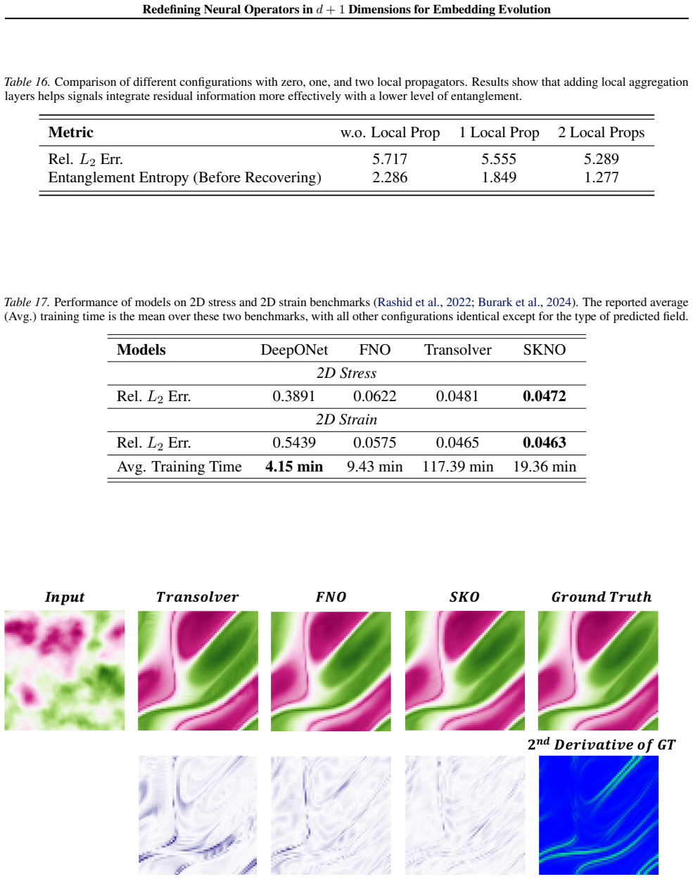
[Sec. 4.1-4.2, Tables 2, 7, 13, 15] The central SOTA claim is not statistically supported. All tables report single runs without error bars, seeds, or code, and several margins over the best baseline are very small (e.g., Burgers 5.475e-4 vs 6.479e-4 in Table 2; shallow-water 0.0027 vs 0.0030 in Table 13; stress 0.0472 vs 0.0481 in Table 17). In addition, the main comparisons are not strictly budget-matched: SKNO uses 4+1 layers (four global propagators plus one local propagator) on Darcy, Navier-Stokes, and Rayleigh-Taylor, whereas FNO uses 4 layers (Table 7), and the local propagator adds an untruncated module. Please report mean and standard deviation over at least three seeds, and release the code and data so that the reported single-run numbers can be independently verified.

minor comments (6)

[Title] The title contains a spacing error: "ind+ 1Dimensions" should read "in d+1 Dimensions".
[Sec. 2.1, Eq. (6)] In the definition of D_mu, the index range "mu_{-Np/2},...,mu_{Np/2}" is incomplete; it should specify the ordering of the DFT frequencies, e.g., "mu_{-Np/2},...,mu_{Np/2-1}" for an even grid.
[Fig. 1 caption] The phrase "a group of Schrödinger / convection equations" is grammatically awkward; consider rephrasing to "a family of uncoupled Schrödinger equations (after Fourier transform in p) and a family of uncoupled convection equations (after Fourier transform in x)".
[Sec. 4.2 and Appendix B, paragraph on spectral decay] The sentence "As shown in Fig. 5 (Li et al., 2021) which illustrates the spectral decay of truncation modes" appears to cite the reference for its own figure; if Fig. 5 is the paper's own figure, the citation should be removed or moved to the text.
[Appendix D, Theorem D.4, Eqs. (46)-(53)] Several equations have unmatched parentheses (e.g., "Grad(bV^(SKNO)_{L-1})_{ij} =" in Eq. (47) is missing a closing bracket). Please carefully proofread the display math.
[Appendix B, "Averaging Neural Operator on Dp"] The reference to "ANO (Lanthaler et al., 2025)" seems inconsistent with the content of the cited paper (which is about universality of nonlinear operators); please verify that the reference supports the averaging-operator claim.

Circularity Check

0 steps flagged · score 0.0 of 10

No significant circularity: SKNO's benchmark results are empirical and self-contained; the d+1 Schrödingerisation framing is motivation, not a fitted prediction.

full rationale

The central claims of the paper are empirical relative-L2 comparisons (Tabs 1, 2, 13, 15) of models trained end-to-end on independent train/test splits under the relative-L2 loss (Eqs. 16–17). No quantity in the Schrödingerisation derivation (Example 1, Eqs. 1–6) is fitted to test data and then reported as a prediction: lifting w(p), recovering χ(p), Fourier weights Ã, and bias b are ordinary learned network parameters, and the d+1 framework (Eqs. 7–10) defines the architecture family rather than supplying its fitted values. The only overlapping-author citation (Li et al., 2025, cited in the introduction for the context that NOs can outperform common NNs) is not load-bearing for SKNO's design or for any benchmark result; the load-bearing theory citations are external (Jin et al. for Schrödingerisation; Kovachki et al. 2021 for universal approximation). Appendix Theorem D.3's inequality follows from the definitional set inclusion H_FNO⊂H_SKNO ('Since H_FNO⊂H_SKNO, the supremum over H_SKNO cannot be smaller...'), which is a best-case superset statement, not an empirical prediction and not the source of the reported SOTA numbers. The Table 1 comparison may be confounded by SKNO's extra local differential operator, but a baseline confound is an external-validity/correctness risk, not a circular reduction: the error gaps are not equal by construction to the fitted parameters. Under the quoted-evidence standard, no circular step is present.

Assumptions & free parameters 3 free parameters · 4 assumptions · 2 invented entities

The central claim rests on standard operator-learning theory, a rank-1 lifting assumption, the specific linear-PDE parameterization along p, and the asserted expressivity inclusion H_FNO ⊂ H_SKNO. The learned network weights are fitted to training data, but the architectural choices (Np, modes, Δt) are hand-chosen. The auxiliary dimension is a model construction, not a physically evidenced entity.

free parameters (3)

Auxiliary grid size Np = 24 to 32 in main experiments; 4 to 16 in linear-block comparisons
The number of grid points along the auxiliary dimension is a hand-chosen capacity parameter that directly controls the expressiveness of the p-dimension Fourier operator. The paper tunes Np per benchmark (Tab. 7) without a principled selection rule.
Number of Fourier modes (truncation) = 1 to 16 depending on benchmark
The spectral truncation in Eq. 11 is set per benchmark; this is a standard hyperparameter but affects the reported accuracy, and no sensitivity analysis is given.
Step size Δt = 1
Eq. 14 sets Δt=1 'for notational simplicity' and notes it can be learnable or tuned, but all experiments use Δt=1. The Euler discretization of Eq. 13 is a modeling choice with no validation.

assumptions (4)

standard math Universal approximation theorem for neural operators (Kovachki et al., 2021) applies to the d+1 dimensional spectral construction
Invoked in Appendix D to assert SKNO is a universal approximator; the paper relies on this rather than proving the d+1 extension from scratch.
domain assumption The lifting v0(x,p) = w(p)^T a(x) is a sufficiently expressive preparation of the d+1 dimensional signal
Eq. 7 assumes a separable (rank-1) lifting is enough to represent the initial auxiliary state for the solution operator. The paper ablate different P,Q choices in Tab. 5 but does not prove the rank-1 form is non-restrictive.
ad hoc to paper The evolution of the embedding along p is governed by a linear PDE of the form Eq. 13 and is faithfully implemented by F_p^{-1} \tilde{A} F_p + b
Sec. 3.2 postulates this parameterization; the paper provides the heuristic alignment with Schrödingerisation but no proof that the learned \tilde{A} can represent the required dynamics on nonlinear benchmarks. This is the central representational assumption.
ad hoc to paper H_FNO ⊂ H_SKNO (SKNO can realize every FNO linear map under the same width budget)
The proof of Theorem D.3 (efficient energy capture) asserts this inclusion without derivation. It is load-bearing for the theoretical claim that SKNO's truncation error is no worse than FNO's.

invented entities (2)

Auxiliary dimension p
purpose: Adds an extra axis to the neural operator domain so that embedding evolution is modeled as a d+1 dimensional operator evolution (Eqs. 7-9).
The p dimension is a mathematical/modeling construction borrowed from Schrödingerisation (Jin et al.); it is not a physical degree of freedom and has no falsifiable handle outside the model's benchmark performance. Its utility is demonstrated only through SKNO's empirical results.
Schrödingerised Kernel Neural Operator (SKNO)
purpose: The proposed architecture that evolves lifted embeddings jointly along x and p via Fourier kernels.
SKNO is a new model class; its value is assessed entirely on the benchmarks in the paper. No independent prediction or external dataset is used to validate the architecture itself.

how reviews work

0 comments

Cite this review

Pith. "Pith review of Reformulating Neural Operators in $d+1$ Dimensions for Embedding Evolution." pith.science (2026). https://pith.science/paper/QF56AU25

@misc{pith2026250511766,
  author       = {Pith},
  title        = {Pith review of: Reformulating Neural Operators in $d+1$ Dimensions for Embedding Evolution},
  year         = {2026},
  howpublished = {\url{https://pith.science/paper/QF56AU25}},
  note         = {Machine review of arXiv:2505.11766}
}

abstract

Neural Operators (NOs) are powerful architectures for learning mappings between function spaces. While most advances focus on refining kernel parameterizations over the $d$-dimensional physical domain, the evolution of lifted embeddings remains underexplored, which often drives models toward computationally expensive embedding-scaling designs to improve approximation. In this paper, we introduce an auxiliary function dimension that models embedding evolution in operator form, thereby reformulating the NO pipeline in $d+1$ dimensions. We instantiate this framework via Fourier-based operators acting jointly on the physical and auxiliary domains, yielding a basis-diversified auxiliary evolution module as an alternative to brute-force embedding scaling. Across more than ten increasingly challenging benchmarks, ranging from the 1D heat equation to the highly nonlinear 3D Rayleigh-Taylor instability, our model consistently achieves the lowest relative $L_2$ error among the evaluated baselines. Crucially, this advantage is empirically supported by (1) controlled budget-aware comparisons against scaled and ablated baselines; (2) robustness under mixed-resolution training and super-resolution inference; and (3) zero-shot generalization to unseen temporal regimes. In addition, we present a broader set of design choices for lifting and recovery operators, demonstrating their impact on our model's predictive performance.

Figures

Figures reproduced from arXiv: 2505.11766 by the authors.

**Figure 1.** A-Schrödingerisation: Classical linear PDEs can be transformed into their d + 1 dimensional version (here d = 1 for visualization) by a warped phase transformation, e.g., heat equation → phase-space heat equation. And it can be represented by a group of Schrödinger / convection equations after taking the Fourier Transform on p / x. B-Neural Operator: Different d dimensional linear operators can be similarly lifted t… view at source ↗

**Figure 2.** When the linear block admits a well-defined operator parameterization, the overall nonlinear approximation can be justified via universal approximation theory (Kovachki et al., 2021). Note that, the concrete implementation of L, whose core component is K in Eq. 8, depends on the specific model design; see Sec. 3.1. Recovering After evolving v(x, p), we take weighted integration on Dp with a learnable function χ(p),… view at source ↗

**Figure 3.** Overview of the Schrödingerised Kernel Neural Operator (SKNO) architecture. The input signal a is lifted to a d+1 dimensional signal v0 through the preparation lifting module. Such a d + 1 dimensional signal evolves through (L − 1) global propagators and one local propagator in Dx, capturing both global and local signal changes. The measuring module recovers the output signal u from evolved vL. Differential Operator… view at source ↗

Figures from the paper (13 more)

**Figure 4.** Figure 4: Evolution along the auxiliary dimension and corresponding neural operator implementations. Left: The target operator L ′ governs the evolution along p. Right: Whereas prior methods rely on discretized matrices at each p location, our model captures this evolution using…

**Figure 5.** Figure 5: Model performance on the Burgers equation with grid size ranging from 128 to 8192. Other Experiments More experiment results and visualizations can be found in the Appendix, mainly including (i) Zero-shot Generalization to Unseen Temporal Regimes: We have shown the SO…

**Figure 6.** Figure 6: Dictionary comparison of FNO and SKNO. We train both models with a sufficiently large recovering budget Np on the Burgers benchmark and visualize the absolute values of the input/output weights, together with the mean energy of the dictionary of pattern fields. While t…

**Figure 7.** Figure 7: Entanglement entropy of intermediate layer outputs. For five randomly selected test cases from the test set, the final entanglement entropy of SKNO is consistently lower than that of FNO, indicating that the (d + 1)-dimensional design of SKNO yields representations tha…

**Figure 8.** Figure 8: Pattern visualization of the 2D Darcy case. According to the discontinuities in the inputs, SKNO learns patterns at different scales. 𝑰𝒏𝒑𝒖𝒕 𝑻𝒓𝒂𝒏𝒔𝒐𝒍𝒗𝒆𝒓 𝑭𝑵𝑶 𝑺𝑲𝑶 (𝒘. 𝒐. 𝒍𝒐𝒄𝒂𝒍) 𝑺𝑲𝑶 𝑮𝒓𝒐𝒖𝒏𝒅 𝑻𝒓𝒖𝒕𝒉 𝟐𝒏𝒅 𝑫𝒆𝒓𝒊𝒗𝒂𝒕𝒊𝒗𝒆 𝒐𝒇 𝑮𝑻 [PITH_FULL_IMAGE:figures/full_fig_p023_8.png]

**Figure 9.** Figure 9: Prediction, error, and second derivative of ground truth visualization for 2D Darcy. The top row shows predictions from different models and ground truth, while the bottom row presents the corresponding error visualizations and the second derivative of the ground truth…

**Figure 10.** Figure 10: Prediction, error, and second derivative of ground truth (GT) visualization for 2D Darcy. 27 [PITH_FULL_IMAGE:figures/full_fig_p027_10.png]

**Figure 11.** Figure 11: Pattern visualization of the 2D Navier-Stokes case. 28 [PITH_FULL_IMAGE:figures/full_fig_p028_11.png]

**Figure 12.** Figure 12: Visualization of the 2D Gray-Scott case. Top: u; Bottom: v. SKNO achieves the lowest error on both. 𝑰𝒏𝒑𝒖𝒕 𝑫𝒆𝒆𝒑𝑶𝑵𝒆𝒕 𝑻𝒓𝒂𝒏𝒔𝒐𝒍𝒗𝒆𝒓 𝑪𝑵𝑶 𝑭𝑵𝑶 𝑺𝑲𝑵𝑶 𝑮𝒓𝒐𝒖𝒏𝒅 𝑻𝒓𝒖𝒕𝒉 𝟐𝒏𝒅 𝑫𝒆𝒓𝒊𝒗𝒂𝒕𝒊𝒗𝒆 𝒐𝒇 𝑮𝑻 [PITH_FULL_IMAGE:figures/full_fig_p029_12.png]

**Figure 13.** Figure 13: Visualization of the 2D Shallow-Water case with randomly mixed training data at different resolutions, evaluated at the highest resolution. 29 [PITH_FULL_IMAGE:figures/full_fig_p029_13.png]

**Figure 14.** Figure 14: Visualization of the 3D Rayleigh–Taylor instability case. All slices are parallel to the coordinate planes, and their intersection points are chosen as the grid points nearest to the center of the box. We show a representative extreme case, namely predicting the outpu…

**Figure 15.** Figure 15: Visualization of zero-shot predictions at future time steps. For the 2D incompressible Navier–Stokes with viscosity 1 × 10−4 (Li et al., 2021), all models are autoregressively evaluated over the twenty time steps following the input time. SKNO maintains its state-of-t…

**Figure 16.** Figure 16: Visualization of paired output weights and pattern fields. All pattern fields are sorted in descending order of the absolute value of their associated output weights, and values marked in red lie below the contribution threshold of 10−3 . Even with the same sufficient…

Discussion (0). Continue with ORCID to comment.

Reference graph

Works this paper leans on

3 extracted references · 3 canonical work pages

[1]

Approximating an operatorM is equivalent (via the Fourier-conjugate decomposition) to approximating the conjugate mapping(s){ cMi}kx i=1 (and, after also Fourier-transforming inp, the conjugates{ fcMi})

work page
[2]

01") denotes the output after theL0 and before theσ0 betweenv0 andv1, whereas a single-digit index (e.g.,

The forward DFT/frequency-projection and the inverse discrete transform admit neural operator approximation on the spectral domain (See Lemma 7 and Lemma 8 in (Kovachki et al., 2021), hence the operator learning problem reduces to a finite-dimensional neural-network approximation on the compact coefficient sets ˆVi, ˜ˆVi. In particular, treating the auxil...

work page arXiv 2021
[2021]

adding one dimension

which illustrates the spectral decay of truncation modes, our chosen benchmarks 6 and 7 contain significantly more high-frequency modes than simpler benchmarks such as 3 or other incompressible NS benchmarks withν >1×10 −4. To further evaluate the capability of these efficient and lightweight neural operators in capturing complex non-linear dynamics in 3D...

work page 2021

Pith tools

Reviewed August 15, 2026 · model on record in the stance chip above.

[1] [1]

Approximating an operatorM is equivalent (via the Fourier-conjugate decomposition) to approximating the conjugate mapping(s){ cMi}kx i=1 (and, after also Fourier-transforming inp, the conjugates{ fcMi})

work page

[2] [2]

01") denotes the output after theL0 and before theσ0 betweenv0 andv1, whereas a single-digit index (e.g.,

The forward DFT/frequency-projection and the inverse discrete transform admit neural operator approximation on the spectral domain (See Lemma 7 and Lemma 8 in (Kovachki et al., 2021), hence the operator learning problem reduces to a finite-dimensional neural-network approximation on the compact coefficient sets ˆVi, ˜ˆVi. In particular, treating the auxil...

work page arXiv 2021

[3] [2021]

adding one dimension

which illustrates the spectral decay of truncation modes, our chosen benchmarks 6 and 7 contain significantly more high-frequency modes than simpler benchmarks such as 3 or other incompressible NS benchmarks withν >1×10 −4. To further evaluate the capability of these efficient and lightweight neural operators in capturing complex non-linear dynamics in 3D...

work page 2021