Pith. sign in

REVIEW 4 major objections 5 minor 12 references

Pseudo-Isotopy and Diffeomorphisms of the 4-Sphere I: Loops of Spheres

T0 review · 4 major / 5 minor · reviewed 2026-08-15 · deepseek-v4-flash

Pith's one-line read A new mod-2 invariant detects loops of embedded 2-spheres in connected sums of S2×S2 that cannot be homotoped into the light-bulb space.

desk verdict A genuinely new geometric invariant for loops of 2-spheres in #^k(S^2×S^2), backed by a lot of careful single-eye machinery, but the supplied text does not contain the proof of well-definedness on homotopy classes. read the letter →

arxiv 2505.12088 v2 pith:6Y3SYUTC submitted 2025-05-17 math.GT

classification math.GT MSC 57R3557R5257R5057N37
keywords Smale4-spherediffeomorphismpseudo-isotopyloopsofembedded2-spheresembeddingspacesWhitneydiscscodimension-2
verification ladder T0 review T1 audit T2 compute T3 formal

The pith

A machine-rendered reading of the paper's core claim, the machinery that carries it, and where it could break.

The reading

This paper establishes a new homotopy obstruction for loops of embedded 2-spheres in $S^2\times S^2$ and in connected sums $\#^k(S^2\times S^2)$. For each $k$ it constructs a surjective homomorphism $I:\pi_1(\mathrm{Emb}(\sqcup^k S^2,\#^k(S^2\times S^2)),R_{\mathrm{std}})\to\mathbb{Z}_2^k$ that vanishes on all loops coming from the light-bulb embedding space $LB$. The $i$-th coordinate is computed by putting a loop in finger-first form and summing, mod 2, the interior intersections between ordered finger and Whitney discs in the $i$-th eye. The main work is showing that this count is unchanged under every allowable deformation of the loops and of the disc systems. If the proof is correct, the invariant gives a first codimension-2 example in simply connected 4-manifolds of sphere loops that are not disc-born and that remain nontrivial under stabilization.

What carries the argument

The central object is the finger/Whitney system: at the middle time of a finger-first loop, complete sets $F$ and $W$ of finger and Whitney discs pair the intersections between the moving spheres and the fixed standard spheres. The invariant is carried by the mod-2 intersection matrix $|f_p\cap w_q|$ for $p\le q$ after an embedded-arc normalization. To make this independent of choices the paper proves a sequence of invariance results: disc slides and switchings convert immersed arc data to embedded arc data; Clifford tori and $H_2$-equivalence absorb the ambiguity of normalizations and slides; restandardization maps cover finger twisting, braiding, spinning, and $SO(3)$-twists; and Theorem 6.29 classifies the five ways finger/Whitney systems change under generic 2-parameter homotopies: disc slides, sphere slides, birth/death moves, $x_3$-moves, and saddle moves.

What would settle it

Take the loop built in Example 0.9 from a finger disc $f$ and a Whitney disc $w$ obtained by tubing the standard Whitney disc $w'$ to a 2-sphere linking $f$; the paper computes $I=1$. The theorem would be false if this loop could be homotoped, relative to its basepoint, into the light-bulb space $LB$, because then the kernel condition would force $I=0$. Equally decisive would be finding a 2-parameter deformation of finger-first loops whose finger/Whitney systems differ by an operation not among the five moves in Theorem 6.29 and for which the mod-2 count changes.

Watch

Extended reading notes

Core claim

Theorem 0.3 asserts the existence, for every $k$, of a surjective homomorphism $I$ from $\pi_1(\mathrm{Emb}(\sqcup^k S^2,\#^k(S^2\times S^2)),R_{\mathrm{std}})$ to $\mathbb{Z}_2^k$ whose kernel contains all classes represented by loops in $LB$. A loop with image $(x_1,\dots,x_k)$ gives, upon adjoining a constant extra sphere in a new $S^2\times S^2$ summand, a loop with image $(x_1,\dots,x_k,0)$. Consequently there exist homotopically nontrivial loops that cannot be realized by loops of embedded 2-discs extended through the light-bulb theorem and that stay nontrivial when the number of summands is increased. The invariant is defined by representing a loop as a finger-first isotopy, collecting the finger discs $F$ and Whitney discs $W$ at the halfway time, ordering them along the immersed intersection arc, and taking the mod-2 sum $\sum_{p\le q}|f_p\cap w_q|$ eye by eye.

Load-bearing premise

The whole well-definedness argument rests on Theorem 6.29 being a complete list: any two finger/Whitney systems for homotopic finger-first loops are related by isotopy and the five listed moves, a fact whose final invariance proof is deferred to Section 7.

Editorial extensions

If this is right

  • The surjectivity of $I$ yields $2^k$ distinct homotopy classes of loops of $k$ spheres based at $R_{\mathrm{std}}$, one for each vector in $\mathbb{Z}_2^k$.
  • Loops with nonzero $I$ cannot be homotoped into $LB$, so they do not arise from loops of embedded 2-discs by light-bulb moves.
  • Stabilization preserves nontriviality: adding a constant extra sphere in a new $S^2\times S^2$ summand appends a zero coordinate, so a nonzero class remains nonzero as $k$ increases.
  • For relative classes based at $LB$, Theorem 6.29 gives a complete calculus: such a class is trivial exactly when its finger/Whitney system can be reduced to the trivial system by the five $FW$-moves, which is the natural starting point for constructing smooth 4-dimensional pseudo-isotopy invariants.

Reading between the lines

Editorial extensions of the paper, not claims the author makes directly.

  • The five-move calculus is likely useful beyond $S^2\times S^2$: any quantity defined from finger/Whitney systems that is invariant under the five moves would produce a homotopy invariant of relative embedding classes in other closed 4-manifolds; testing this in $Y\#^k(S^2\times S^2)$ for a general $Y$ is a natural next step.
  • Because the invariant is valued in $\mathbb{Z}_2^k$ and is stable under adding summands, it may be compatible with stabilization maps in embedding spaces; the paper records the append-zero behavior but does not determine whether $I$ factors through a stable homotopy group.
  • The same mod-2 counting might apply to loops of higher-genus surfaces in 4-manifolds once analogues of finger-first position and the five moves are established; the local $FW$-germ analysis in Section 6 is developed for a general surface $R$ in a general 4-manifold $X$.
Share X Bluesky LinkedIn Reddit HN

Signed reviews

No signed human review yet.

Editorial analysis

A structured set of objections, weighed in public.

Desk editor's note, referee report, and a circularity audit.

Referee Report

4 major / 5 minor

Summary. The paper introduces a codimension-2 invariant of loops of embedded 2-spheres in #^k(S^2×S^2). For a loop in finger-first position with a finger/Whitney system, it defines I_j as the mod-2 sum of intersections between ordered finger and Whitney discs pairing the j-th red and green spheres, and I=(I_1,...,I_k). The main theorem (Theorem 0.3) asserts that I is a surjective homomorphism on π_1(Emb(⊔^k S^2, #^k S^2×S^2), R_std), vanishes on loops in the light-bulb subspace, and is natural under stabilization by an extra constant sphere. Sections 2–4 develop the single-eye case and prove independence of the auxiliary choices for a fixed finger-first representative; Section 5 sketches the multi-eye extension; Section 6 analyzes generic 2-parameter families and identifies five moves relating finger/Whitney systems. The text repeatedly defers the final homotopy-invariance proof to a Section 7 that is not present in the supplied manuscript. The paper also outlines intended applications to pseudo-isotopy and to the existence of an exotic element in Diff^+(S^4) in a sequel.

Significance. If Theorem 0.3 is established, the result is a significant advance in simply connected 4-dimensional embedding-space theory: it produces homotopically nontrivial loops of spheres that do not come from loops of discs in light-bulb position, with a stabilization property that is absent from earlier constructions. The invariant is a direct, parameter-free geometric intersection count with no fitted constants, and the single-eye development contains a substantial and careful body of technical lemmas. Example 0.9 provides a concrete and checkable nontrivial loop. However, as submitted, the central theorem is conditional on a missing invariance proof and on the completeness of the five-move classification, so the significance can be certified only after the deferred material is supplied.

major comments (4)
  1. [§0, Definition 0.7; §7 (missing)] The definition of I([α]) is made after choosing a finger-first EA representative, and Sections 2–4 establish independence of choices within such representatives. The step from representatives to a well-defined homotopy invariant is deferred: the introduction states 'In §7 we show that all such operations give a well defined invariant, thereby completing the proof,' but Section 7 is not present in the supplied manuscript. Consequently Theorem 0.3 is not established in the submitted text. This is load-bearing, and the missing proof must be supplied before the central claim can be assessed.
  2. [Theorem 6.29 and §6.7] The completeness of the five-move description is the linchpin connecting the local invariant to the homotopy class [α], but its proof is an outline rather than a complete argument, and no invariance of I under the x3-move or the saddle move is verified here; the introduction explicitly defers this to §7. In particular, saddle moves can change the pairing or order of the discs that contribute to the mod-2 sums, and the reader is not shown why the sums are unchanged when cross discs are present. This missing verification is load-bearing for Theorem 0.3.
  3. [§5] The multi-eye generalization is presented as a sequence of 'Comments on' the single-eye lemmas rather than complete proofs, e.g. 'Comments on Proposition 3.24', 'Comments on Lemma 3.33', 'Comments on Lemma 3.35', 'Comments on Lemma 3.42', and 'Comments on Lemma 3.45'. Since Definition 0.7 deliberately ignores cross terms and I_j is defined eye-by-eye, one needs an explicit proof that cross discs do not affect the mod-2 upper-triangular sums under each restandardization and each FW-move. The text asserts this but does not fully demonstrate it in the multi-eye setting.
  4. [Remark 4.24(ii) and Proposition 4.2] The proof of Proposition 4.2 uses Lemma 7.9 to add a new finger and concludes I(F,W)=I(F1,W1); Remark 4.24(ii) states that this lemma is given in Section 7. Since Section 7 is absent from the submitted manuscript, Proposition 4.2 is incomplete. As Proposition 4.2 is part of the well-definedness chain for the invariant, this dependence must be supplied before the proof is complete.
minor comments (5)
  1. [§6, opening paragraph] The text refers to 'Theorem 6' when it appears to mean Theorem 6.23; please correct the cross-reference.
  2. [§5.4 heading] The heading 'Propositin 4.2' contains a typo and should read 'Proposition 4.2'.
  3. [Construction 6.14 and §6.4.2] There are small typos: 'vector feild' should be 'vector field' and 'vise versa' should be 'vice versa'.
  4. [Remark 4.24(ii)] The remark references Lemma 7.9 without stating it; if that lemma is to be used, its statement and proof must appear, not merely be promised for later.
  5. [§6.7.5] The supplied text breaks off mid-sentence in the saddle-move subsection; if this reflects the submitted version rather than an artifact of transmission, the saddle-move analysis is incomplete and must be restored and integrated with the invariance proof.

Circularity Check

0 steps flagged · score 0.0 of 10

No circularity found: the invariant is a direct geometric mod-2 intersection count, not a fitted parameter or a renamed input; the main caveat is that the supplied text omits the deferred Section 7 proof, which is a completeness risk rather than a circular reduction.

full rationale

I can exhibit no equation or construction by which the paper's prediction is equivalent to its input. Definition 0.7 defines I_j([α]) directly as sum_{p≤q} |f_p∩w_q| mod 2 from a finger/Whitney system, with no fitted constants, no assumed target values, and no self-referential definition of the loop class being detected. The paper's actual burden is well-definedness, and it repeatedly proves invariance under disc slides, Clifford tori, switchings, restandardizations, and orderings (e.g. Proposition 2.19, Proposition 3.24, Propositions 4.1–4.2, and the multi-eye versions in §5) rather than assuming it. Theorem 6.29 is presented as a normal-form statement about how finger/Whitney systems for homotopic paths differ via five FW-moves, and the text explicitly says the final invariance under these moves is shown in Section 7: 'In §7 we show that all such operations give a well defined invariant, thereby completing the proof.' In the supplied full text Section 7 is not present and §6 ends mid-discussion of the saddle move, so the x3- and saddle-move invariance checks cannot be verified here. I flag this as an omitted proof and a correctness/completeness risk, not as circularity. Cited prior work, including Quinn's embedded-arc condition and the authors' [Gab20] and [Gab22] results, is external geometric input; Quinn's EA condition is re-proved in Construction 6.24, and the paper explicitly distances itself from Quinn's Disc Replacement Criterion in Remark 0.10. Thus the derivation chain does not reduce to its own output by construction.

Assumptions & free parameters 0 free parameters · 3 assumptions · 0 invented entities

The central invariant is self-contained once the cited Quinn and Gabai inputs are accepted. No numerical parameters are fitted, and no new physical entities are postulated. The main external inputs are low-dimensional topology facts from Quinn, Budney-Gabai, and Gabai.

assumptions (3)
  • domain assumption Every loop of embedded 2-spheres admits a finger-first representative with a finger/Whitney system in embedded arc position (EA), as asserted by Quinn.
    Used to define I in Definition 0.7 and to reduce all loops to standard finger/Whitney data; cited to [Qui86, §4]. The paper notes a nearby Quinn lemma is suspect, so this is a load-bearing external input.
  • standard math Generic 2-parameter families of embeddings can be modeled by stable maps with folds, cusps, and an FW-vector field that extends the local finger/Whitney germs.
    Section 6 builds the five-move classification on this singularity-theoretic framework; the authors state transversality and stable map results without full proof, treating them as standard background.
  • domain assumption Geometrically dual embeddings can be isotoped to the standard unlinked embedding inside the class of geometrically dual embeddings.
    Used to close loops after finger/Whitney moves in Example 0.9 and Notation 1.3; cited to [Gab20].

how reviews work

0 comments
Cite this review

Pith. "Pith review of Pseudo-Isotopy and Diffeomorphisms of the 4-Sphere I: Loops of Spheres." pith.science (2026). https://pith.science/paper/6Y3SYUTC

@misc{pith2026250512088,
  author       = {Pith},
  title        = {Pith review of: Pseudo-Isotopy and Diffeomorphisms of the 4-Sphere I: Loops of Spheres},
  year         = {2026},
  howpublished = {\url{https://pith.science/paper/6Y3SYUTC}},
  note         = {Machine review of arXiv:2505.12088}
}
abstract

We introduce new methods in pseudo-isotopy and embedding space theory. As an application we introduce an invariant that detects nontrivial loops of embedded 2-spheres in $S^{2} \times S^{2}$ and in connected sums of $S^{2} \times S^{2}$. that cannot be homotoped to loops of spheres dual to the standard horizontal spheres. In the sequel [GGH], we will use these techniques to expand upon the applicability of the invariant and prove $\operatorname{Diff}^{+}(S^{4})$ has an exotic element.

Figures

Figures reproduced from arXiv: 2505.12088 by the authors.

Figure 1
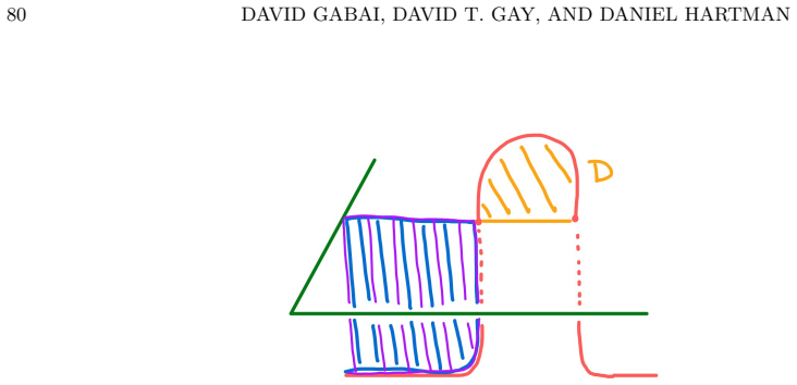
Figure 1. The Key Example ii) The multi-index I([α]) is an invariant of loops of multi-spheres while I([α]) is the pseudo-isotopy invariant of [GGH]. iii) While Quinn’s proof that [α] has a representative α ∈ EA is elementary, we need to do it in a controlled way. Examples 0.9. i) [PITH_FULL_IMAGE:figures/full_fig_p004_1.png] view at source ↗
Figure 2
Figure 2. G-Disc Sliding wi over wj along ω If W and W′ (resp. F and F ′ ) have the same boundary germs, then a disc slide on W (resp. F) naturally corresponds to one on W′ (resp. F ′ ). We say that (F2, W2) is obtained from (F1, W1) by a disc slide if exactly one of F2 or W2 is obtained that way. Define T G wj , the G-normal torus to ∂K, to be the tube about ∂K disjoint from G. In an analogous manner define T R wj . Lemma 2.… view at source ↗
Figure 3
Figure 3. Constructing a Twisted G-Whitney Disc Slide the same ∂ germ as w ′ i , then ˆw ′ i is obtained from w ′ i by doing cut and past with n copies of T G wj . Since we are working with Z2 intersection numbers what matters is the parity of p. ii) On the other hand if ˆwi or ˆwj are obtained by twisting near R, then the corresponding G-disc slide is unchanged. Definition 2.6. Recall that if c is a point of transverse inter… view at source ↗
Figures from the paper (53 more)
Figure 4
Figure 4. Figure 4: Going from Immersed Arc to Embedded Arc Position Lemma 2.14. Let F, W be untwisted sets of discs such that (F ∪ W) ∩ R is the embedded union of circles and possibly an arc. Let (F ′ , W′ ) be obtained from (F, W) by either an untwisted G-disc slide or by an R-twist of …
Figure 5
Figure 5. Figure 5: Framed Finger Form assume that the positive bundle of R is standard in a 2-disc containing the fingers and a0. Since R has trivial normal bundle we can isotope N(R) to have the standard framing on all of N(R). Note that if the positive bundle of G was already standard,…
Figure 6
Figure 6. Figure 6: Rotating a Finger to Correct the Positive Framing Definition 3.13. The κ of Lemma 3.12 is called a standardizing map. Corollary 3.14. Given a complete ordered set [PITH_FULL_IMAGE:figures/full_fig_p018_6.png]
Figure 7
Figure 7. Figure 7: a) 3-Switch b) 2-Switch Lemma 3.17. Given (F, W) with W ordered and untwisted, then the switch out discs are canonically chosen and there is a corresponding reordering wi1 < wi2 < · · · < win of the elements of W, called the F-reordering with the property that all the …
Figure 8
Figure 8. Figure 8: Constructing Wˆ Given Wˆ and an ordering on W, the relevant data for determining an order induced k￾switch is first, for each i picking out a single wj in the i’th cycle and second, ordering these wj ’s. For a given order on W one readily constructs the desired order i…
Figure 9
Figure 9. Figure 9: a) Constructing W1 b) Constructing W2 i) The IA ordering on ((F ∪ W1 ) ∩ (σi \wi)) ∪w 1 i is induced from the linear order on that immersed segment having w 1 i as the maximal element. ii) If r < s, then all elements in σs ∪ w 1 s appear before elements in σr ∪ w 1 r .…
Figure 10
Figure 10. Figure 10: a) W has the standard ordering b) The IA Ordering: f1 < w∗ 2 < f2 < w∗ 3 < f3 < w∗ 1 < f4 < w∗ 4 Definition 3.23. Given R and G in framed finger form, then a restandardization map is the time 1 map ψ of an ambient isotopy that fixes G ∪ R setwise, fixes the standard W…
Figure 11
Figure 11. Figure 11: Two Views of the Solid Finger σF b) C ∩ G ̸= ∅ and C ∩ R = ∅: Here C ∩σ is an arc with one endpoint on G and N(C)∩ G is an arc with one endpoint on ∂eσ. See [PITH_FULL_IMAGE:figures/full_fig_p023_11.png]
Figure 12
Figure 12. Figure 12: Types of Components of a Whitney germed f in a Solid Finger [PITH_FULL_IMAGE:figures/full_fig_p024_12.png]
Figure 13
Figure 13. Figure 13: b) shows ψ(w ∗ i ). The effect of G-finger twisting on G is a Dehn twist on ∂N(wi) ∩ G. We can arrange that the effect on R is a Dehn twist on σRF is also a Dehn twist which in particular fixes the normal framing of R setwise. Note that ψ is isotopic to id via an isot…
Figure 14
Figure 14. Figure 14: Invariance under G-Finger Twisting We prove ˆI(F, W1) = ˆI(F, W3). First consider the case j < k. By Lemma 3.22 the IA ordering on (F, W3) contains the following linear sequence w 3 j+1 < ϕ1 < τ1 < ϕ2 < τ2 < · · · < ϕm < w3 j where {ϕ1, · · · , ϕm} = F ∩ ω and {τ1, · …
Figure 15
Figure 15. Figure 15: G-Braiding Proof. We will prove this with W1, W2 finger framed and F Whitney framed. Note that αij is obtained by banding αi to αj along the thin band bij ⊂ G with core β. We assume that bij is transverse to W1 ∩ G and call a component of bij ∩ W1 a middle arc. Up to …
Figure 16
Figure 16. Figure 16: a) ψ(w 1 1 ) b) After the boundary compression Case 1 : There are fp, fq ∈ F that respectively match wi , wj ∈ W and j ≤ k [PITH_FULL_IMAGE:figures/full_fig_p028_16.png]
Figure 17
Figure 17. Figure 17: Very Local View of the SO(3) Twist Lemma 3.44. If ψ is the result of a SO(3)-twist about σi and W1 is the result of a k-switch to W and W2 = ψ(W1), then w 2 j = ψ(w 1 j ) unless w 1 j is a switch disc and j = i or j = i + 1 [PITH_FULL_IMAGE:figures/full_fig_p031_17.png]
Figure 18
Figure 18. Figure 18: b). Second, modify as in [PITH_FULL_IMAGE:figures/full_fig_p032_18.png]
Figure 19
Figure 19. Figure 19: A G-Disc Clasp - The full w4 clasp disc is not shown a2i and a2j−1. By pushing w a i (resp. w a j ) slightly into the future (resp. past) near β we obtain disjoint discs w b i , wb j each of which intersects R at one point in its interior. We eliminate these intersect…
Figure 20
Figure 20. Figure 20: The Construction of W′ [PITH_FULL_IMAGE:figures/full_fig_p037_20.png]
Figure 21
Figure 21. Figure 21: Possibilities for ϕ(W′ ) where W′ arises from γ4,9 Case 2 : |γij ∩ W| = 2. Proof of Case 2 : We give the proof for t a R-Dehn twist about γ4,8, the other subcases being similar. Here W′ is constructed as in [PITH_FULL_IMAGE:figures/full_fig_p038_21.png]
Figure 22
Figure 22. Figure 22: The Construction of W′ - The full w ′ 4 is not shown G R S1 S2 S3 R3 R1 R2 [PITH_FULL_IMAGE:figures/full_fig_p039_22.png]
Figure 23
Figure 23. Figure 23: Free Generators for H2(S 2 × S 2 \ (N(G ∪ R))) Lemma 4.17. If D is a properly embedded disc in E, then H2(E, ∂D) is freely generated by D, R1, · · · , Rn, S1, · · · , Sn. □ Lemma 4.18. i) If Di is a Whitney disc whose ∂-germ coincides with that of the standard Whitney…
Figure 24
Figure 24. Figure 24: Constructing the 5-Switch W∗ 2 for W2 IA order on (F, W∗ i ) for i = 1, 2. The figures shows (F ∪ W∗ i ) ∩ G with both the old and new names of the discs. f1 f2 f3 f4 f5 w1 1 w2 1 w3 1 w4 1 w5 1 f1 f2 f3 f4 f w1 5 2 w2 2 w5 2 f1,1 f1,2 f1,3 f f1,5 1,4 f f2,5 f2,3 f2,4…
Figure 25
Figure 25. Figure 25: The IA Ordering on a) (F, W∗ 1 ) and b) (F, W∗ 2 ) The following result completes the proof of Case 1. Lemma 4.23. For i = 1, 2 the matrices of Tables 6.6 and 6.7 respectively record the values of ⟨fi,p, w∗ i,q⟩ for p ≤ q viewed mod-2, from which we conclude I(F, W1) …
Figure 26
Figure 26. Figure 26: Constructing f 3 2 near S 2 × S 1 × 0 G' R' [PITH_FULL_IMAGE:figures/full_fig_p043_26.png]
Figure 27
Figure 27. Figure 27: Constructing f 3 2 near S 2 × S 1 × −ϵ Fourth, moving further into S 2 × S 1 × t, t < −ϵ we see that the parallel copies of G′ ∩ S 2 × S 1 × t are parallel R ∩ S 2 × S 1 × t and just like R they are capped off with discs within S 2 × S 1 × [−∞, t]. Similarly moving in…
Figure 28
Figure 28. Figure 28: The tube paths, with multiplicity, in R and G EA order. In the EA order the finger discs are denoted f3,1, f3,2, · · · , f3,5. Now each f 3 i comes with its twisting (pi , qi) and an ai where aiSi corrects the framing. There are three types of intersections that contr…
Figure 29
Figure 29. Figure 29: Multi-Eye Framed Finger Form Allowing for multi-components and multi-indices the material from Lemma 3.12 through Definition 3.23 extend to the multi-eye setting. Definition 5.4. A finger from Ri into Gj , with i ̸= j is called a cross finger. A finger (resp. solid fi…
Figure 30
Figure 30. Figure 30: The following image depicts the trace of the family Rt near a finger/Whitney point. In purple we have the cone C(B2 ) and in blue C(B1 ). Their union is the FW germ for the finger/Whitney point [PITH_FULL_IMAGE:figures/full_fig_p055_30.png]
Figure 31
Figure 31. Figure 31: The local interaction between Rs,t and G near a fold singularity for h : Σ → B2 . Each frame shows the configurations of Rs,t and G in a 3-ball slice of a 4-ball neighborhood around the point Rs0,t0 (p). The middle frame depicts the configuration corresponding to Rs0,…
Figure 32
Figure 32. Figure 32: The local interaction between Rs,t and G near a cusp singularity for h : Σ → B2 . Each frame shows the configurations of Rs,t and G in a 3-ball slice of a 4-ball neighborhood around the point Rs0,t0 (p). The middle frame depicts the configuration corresponding to Rs0,…
Figure 33
Figure 33. Figure 33: Local model for critical points of Σ. by (s, t) with t the path parameter and s the homotopy parameter. We will denote by Hs the path of embeddings given by restricting H to the line {s} × [0, 1]. Let Ls denote Σ ∩ {s} × [0, 1] × R and hs the function h|Ls . Finally, …
Figure 34
Figure 34. Figure 34: This figure illustrates the overlap of the supports for the vector fields constructed on [0, 1]2 × X \ ν(Sh) in Construction 6.19 near the inter￾section of tr(H) (in red) and [0, 1]2 × G (in green); in black we shown have the support of V1, in orange the support of V2…
Figure 35
Figure 35. Figure 35: Local deformation A similar story holds for Deformation 3. In order to move the family of finger moves past the cusp, we need to make sure that when we extend the finger arcs below the index 1 fold, they miss the corresponding finger disc for the index. The local mode…
Figure 36
Figure 36. Figure 36: Depicted is a subset of the local Cerf graphic for two families of finger moves [PITH_FULL_IMAGE:figures/full_fig_p069_36.png]
Figure 37
Figure 37. Figure 37: Shown is the neighborhood for the family of local finger discs (in blue) and the family extended finger arc (in black). Moreover, the two types of intersections will occur generically for distinct s-parameter values [PITH_FULL_IMAGE:figures/full_fig_p069_37.png]
Figure 38
Figure 38. Figure 38: Shown here is the change in the local disc given by dragging the extended finger arc at s > s0 back to s < s0. The result is that the local disc changes by a G disc slide. arranged the tangent vector of the arc at the boundary to be constant and tangent to the disc at…
Figure 39
Figure 39. Figure 39: Shown is the neighborhood for the local finger disc (in blue) and the intersections of this neighborhood with the extended family of finger arcs (in black) [PITH_FULL_IMAGE:figures/full_fig_p071_39.png]
Figure 40
Figure 40. Figure 40: Here we depict the affect of isotopying the extended family of arcs at s > s0 back to its position at s < s0. The resulting change to the disc is a sphere slide. Definition 6.37. Let f1 and f2 be two framed finger (Whitney) discs pairing off intersections between R an…
Figure 41
Figure 41. Figure 41: The following figure illustrates an example of a birth move. of finger/Whitney discs for the finger/Whitney system at s = 0. Then (R, G, F, W)0 differ from (R, G, F, W)1 by adding (removing) a pair of intersections between R and G and adding (removing) a pair of discs…
Figure 42
Figure 42. Figure 42: Depicted here is the local model for a cusp point. Shown in blue is the corner for some finger/Whitney disc, and how we extend the corner through the cusp singularity. As the rest of the disc is away from the singular set Sh, this figure describes how the finger/Whitn…
Figure 43
Figure 43. Figure 43: Shown are the two possible extensions of the blue disc, depending on whether it is a finger disc or a Whitney disc [PITH_FULL_IMAGE:figures/full_fig_p075_43.png]
Figure 44
Figure 44. Figure 44: On the left depicts the local isotopy of the corner in the neigh￾borhood, arranging so that both the finger and the Whitney disc agree near R ∩ G in the neighborhood. On the right is the other possible configuration of the finger/Whitney data [PITH_FULL_IMAGE:figures…
Figure 45
Figure 45. Figure 45: Shown are the possible extensions through the cusp point locally, depending on which disc is the finger disc and which is the Whitney disc. Case 3: The final case considers when the double point interacts with both a finger disc and Whitney disc. In the local model, t…
Figure 46
Figure 46. Figure 46: Shown is the local Cerf graphic for H near a saddle point. data back, letting s vary from s > s0 to s < s0. The new finger/Whitney discs then cancel each other, and the extended discs return to their previous configuration. Moreover, we can compare the extended system…
Figure 47
Figure 47. Figure 47: Here is an illustration of the possible configurations of the fin￾ger/Whitney data (in blue and purple) in the local neighborhood of the saddle disc D(in yellow). duplicates and becomes two separate arcs: One for the newly created finger move, γ f D, the other for the…
Figure 48
Figure 48. Figure 48: Shown here is an illustration of where the extended data lives. In particular, the Whitney discs for the moves happening at t = 3/4 can be extended to the t = tw level sets, but not necessarly below for s ∈ (s0, s1). A similar statement holds for the finger discs. For…
Figure 49
Figure 49. Figure 49: Shown is a local neighborhood for a saddle disc D pairing of points in R ∩ G with one such point free of all other finger/Whitney data. In blue and purple, we have corners for the finger disc and Whitney disc that pair off the other intersection point [PITH_FULL_IMAG…
Figure 50
Figure 50. Figure 50: Depicted is the extension of the corners, and how the splitting of the finger arc γD affects the corners in the local model. two finger discs can not pair off the same intersection point. We can arrange in the local model that when γ separates, either γw ⊂ wc or γf ⊂ …
Figure 51
Figure 51. Figure 51: Shown is the configurations of the corners for the finger/Whitney data in the local neighborhood of a saddle disc in general [PITH_FULL_IMAGE:figures/full_fig_p081_51.png]
Figure 52
Figure 52. Figure 52: Depict is the sequence of extending the corners across the pa￾rameters (s0, s1) and the affect the splitting of the finger arc γD has on the data. shall assume that, after a local isotopy, the corresponding positive and negative cor￾ner data agree, as shown in [PITH_…
Figure 53
Figure 53. Figure 53: Shown is the local change to the boundaries of the fin￾ger/Whitney discs under the x 3 -move [PITH_FULL_IMAGE:figures/full_fig_p087_53.png]
Figure 54
Figure 54. Figure 54: Shown is an illustration of the changes in the finger/Whitney discs that intersect the local neighborhood of the saddle disc D under the saddle move. created either. Therefore, ˆIis<s0 = ˆIi(∆s>s0 ). What remains is the disc slides needed to get to EA. We can perform …
Figure 56
Figure 56. Figure 56: Here is an example of the boundaries of the discs after switching together with the induced IA ordering. The top row indicates the configu￾ration of the discs locally near D in Ri and Gi while the second row is the configurations after the saddle move. Ii(W, F). As su…
Figure 57
Figure 57. Figure 57: On the left shows the extended arc for the upper finger arcs (in black) and the lower Whitney arcs (in blue). On the right we see the finger/Whitney system after the deformation into finger-first postion. same sequence of disc slides on ∆s<s0 as we do with ∆s>s1 , add…

Discussion (0). Continue with ORCID to comment.

Reference graph

Works this paper leans on

12 extracted references · 3 canonical work pages

  1. [1]

    [Art25] E. Artin. Zur Isotopie zweidimensionaler Fl¨ achen imR4. Abh. Math. Sem. Univ. Ham- burg 4.1 (1925), pp. 174–177. issn: 0025-5858,1865-8784. doi: 10.1007/BF02950724. url: https://doi.org/10.1007/BF02950724 (p. 1). [Bro67] W. Browder. Diffeomorphisms of 1-connected manifolds. Trans. Amer. Math. Soc. 128 (1967), pp. 155–163 (p. 5). [BG19] R. Budney ...

  2. [6]

    With English and French prefaces

    Ast´ erisque. With English and French prefaces. Soci´ et´ e Math´ ematique de France, Paris, 1973, pp. i+275 (pp. 1, 5, 6). [HO] S. Hirose and G. Omori. Finite Presentations for the balanced superelliptic mapping class groups. Preprint (p. 34). [Igu21] K. Igusa. Second obstruction to pseudoisotopy I

  3. [10]

    url: https://doi.org/10.2140/gt.1999.3.103 (p

    2140/gt.1999.3.103. url: https://doi.org/10.2140/gt.1999.3.103 (p. 1). [Hat83] A. Hatcher. A proof of the Smale conjecture, Diff( S3)≃ O(4). Ann. of Math. (2) 117 (1983), pp. 553–607 (p. 55). [HW73] A. Hatcher and J. Wagoner. Pseudo-isotopies of compact manifolds . Vol. No

  4. [11]

    url: https://arxiv.org/abs/2110.09659 (p

    arXiv: 2110.09659 [math.GT]. url: https://arxiv.org/abs/2110.09659 (p. 1). [KM63] M. A. Kervaire and J. W. Milnor. Groups of homotopy spheres. I. Ann. of Math. (2) 77 (1963), pp. 504–537 (p. 5). REFERENCES 93 [Qui86] F. Quinn. Isotopy of 4-manifolds. J. Diff. Geom. 24 (1986), pp. 343–372 (pp. 2, 3, 4, 6, 7, 64, 81, 88, 90). [Sin22] O. Singh. Pseudo-isotop...

  5. [14]

    Springer Science & Business Media, 2012 (p. 56). [GW99] T. G. Goodwillie and M. Weiss. Embeddings from the point of view of immersion theory. II. Geom. Topol. 3 (1999), pp. 103–118. issn: 1465-3060,1364-0380. doi:

  6. [39]

    Princeton University Press, Princeton, NJ, 1990, pp

    Princeton Math- ematical Series. Princeton University Press, Princeton, NJ, 1990, pp. viii+259. isbn: 0-691-08577-3 (p. 2). [Gab21] D. Gabai. Self-Referential discs and the light bulb lemma. Comment. Math. Helv. 96 (2021), pp. 483–513 (pp. 30, 61). [GGH] D. Gabai, D. Gay, and D. Hartman. Diffeomorphisms of the 4-sphere II: general 2-parameter families. In...

  7. [2019]

    url: https://arxiv.org/abs/1912.09029 (pp

    arXiv: 1912.09029 [math.GT]. url: https://arxiv.org/abs/1912.09029 (pp. 1, 2). [Cer61] J. Cerf. Topologie de certains espaces de plongements. Bull. Soc. Math. France 89 (1961), pp. 227–380 (p. 6). [FGHK24] E. Fern´andez, D. T. Gay, D. Hartman, and D. Kosanovi´c. Grasper families of spheres in S2× D2 and barbell diffeomorphisms of S1× S2× I

  8. [2021]

    url: https://arxiv.org/abs/2102.12890 (p

    arXiv: 2102.12890 [math.GT]. url: https://arxiv.org/abs/2102.12890 (p. 6). [GG12] M. Golubitsky and V. Guillemin. Stable mappings and their singularities . Vol

Show all 12 references
  1. [2022]

    url: https://arxiv.org/abs/2212.02004 (pp

    arXiv: 2212.02004 [math.GT]. url: https://arxiv.org/abs/2212.02004 (pp. 6, 7, 9, 17, 23, 36, 42). [GGHKP] D. Gabai , D. T. Gay , D. Hartman, V. Krushkal , and M. Powell . Pseudo- isotopies of simply connected 4-manifolds

  2. [2023]

    url: https://arxiv.org/abs/2311.11196 (pp

    arXiv: 2311.11196 [math.GT]. url: https://arxiv.org/abs/2311.11196 (pp. 4, 6, 70). [Gay21] D. T. Gay. Diffeomorphisms of the 4-sphere, Cerf theory and Montesinos twins

  3. [2024]

    url: https://arxiv.org/abs/2412.07467 (p

    arXiv: 2412.07467 [math.GT]. url: https://arxiv.org/abs/2412.07467 (p. 1). [FQ90] M. H. Freedman and F. Quinn. Topology of 4-manifolds. Vol

  4. [2111]

    url: https://arxiv.org/abs/2111.15658 (p

    15658 [math.GT]. url: https://arxiv.org/abs/2111.15658 (p. 1). [Sma61] S. Smale. Generalized Poincare’s conjecture in dimensions greater than four. Ann. of Math. (2) 74 (1961), pp. 391–406 (p. 5). [Wei99] M. Weiss. Embeddings from the point of view of immersion theory. I. Geom...

Pith tools

Reviewed August 15, 2026 · model on record in the stance chip above.