REVIEW 4 major objections 5 minor 2 cited by
(U)NFV: Supervised and Unsupervised Neural Finite Volume Methods for Solving Hyperbolic PDEs
T0 review · 4 major / 5 minor · reviewed 2026-08-07 · deepseek-v4-flash
Pith's one-line read A neural network that learns the numerical flux of a finite volume scheme cuts error up to tenfold versus Godunov's method while preserving exact conservation.
desk verdict A credible empirical extension of learned finite volume methods with public code, but the abstract oversells ENO/WENO wins and a missing consistency check leaves the 'solver' claim unsettled. read the letter →
The pith
A machine-rendered reading of the paper's core claim, the machinery that carries it, and where it could break.
The reading
What carries the argument
The object that carries the argument is the learned numerical flux $\hat{F}_{i\pm 1/2} = N(u_{i\pm 1/2}(a-1,b))$: a one-dimensional convolutional network that reads a stencil of $a$ spatial cells across $b$ past time steps and outputs the flux through a cell interface. It does the work of the flux function in a classical finite volume scheme, and the conservative update rule $u^{n+1}_i = u^n_i - \frac{\Delta t}{\Delta x}(\hat{F}_{i+1/2} - \hat{F}_{i-1/2})$ then enforces mass conservation exactly, because the flux leaving one cell enters its neighbor whatever the network outputs. The stencil classes $\mathrm{FV}^b_a$ and $\mathrm{NFV}^b_a$ organize the design space, placing Godunov's method in the 3-by-1 class and letting the authors push learned fluxes to 11-by-11 stencils that would be impractical to derive analytically. For the unsupervised variant, the training signal is a weak-form residual loss evaluated cell-wise against 250 compactly supported polynomial test functions of degree 50. The methodological claim is that this one learned object, the flux, carries the entire burden of accuracy, entropy selection, and generalization.
What would settle it
Evaluate any trained NFV at constant states: feed the network a uniform field $u$ in every stencil cell and compare its output $N(u,\ldots,u)$ to the physical flux $f(u)$. If the two disagree while the scheme still appears accurate, then measure the scheme's autoregressive error on a mesh substantially finer than the training mesh; a learned flux that is not consistent should show the error plateauing or growing as the mesh refines, whereas a genuinely consistent scheme would keep converging to the exact entropy solution.
Extended reading notes
Core claim
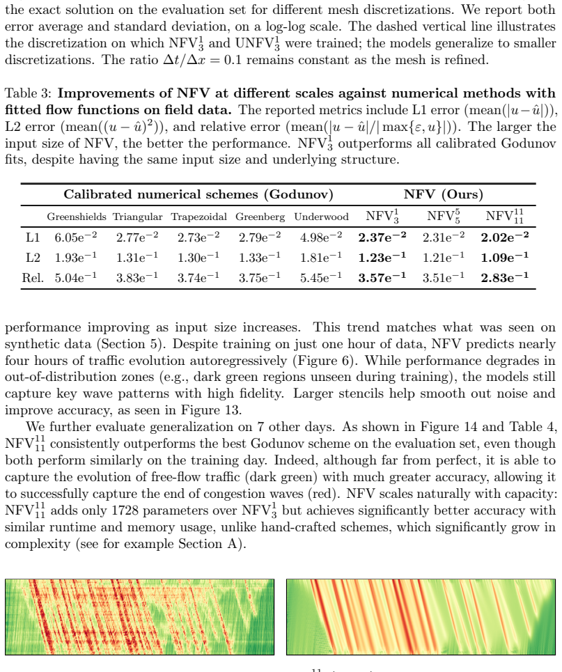
The paper's central claim is that a learned numerical flux is a sufficient upgrade over classical finite volume solvers: replace the hand-derived flux $F(u^n_i, u^n_{i+1})$ with a neural network $N$ applied to an $a$-by-$b$ stencil of neighboring cells and past time steps, keep the exact update $u^{n+1}_i = u^n_i - \frac{\Delta t}{\Delta x}(\hat{F}_{i+1/2} - \hat{F}_{i-1/2})$, and accuracy improves by up to an order of magnitude while conservation remains exact by construction. The claim is made in two settings. In the supervised setting, NFV is trained on Riemann problem solutions and evaluated on harder piecewise-constant initial conditions with ten discontinuities; in the unsupervised setting, UNFV is trained purely against a weak-form residual loss with randomly sampled polynomial test functions, and the paper reports that it converges to the entropy solution across a range of flow functions. The method scales with stencil size — larger stencils such as NFV$^{11}_{11}$ add only modest parameter counts over NFV$^{1}_{3}$ yet cut error substantially — and it transfers to field data: trained on one hour of I-24 MOTION density data, NFV$^{11}_{11}$ beats the best calibrated Godunov fit both on the training day and on seven unseen days. The authors state clearly that no stability or convergence guarantees accompany these empirical results.
Load-bearing premise
The load-bearing premise is that a flux network trained on one family of stencils and equations keeps behaving like a valid numerical flux when the mesh is refined, the flux function changes, or the data is noisy — the network is never constrained to be consistent with the physical flux, and the paper offers empirical evidence but no stability or convergence proof.
Editorial extensions
If this is right
- If the claims hold, standard first-order finite volume solvers can be swapped for a learned flux network with roughly tenfold lower error at nearly identical implementation and runtime cost.
- Larger spatiotemporal stencils improve accuracy, which suggests that learned schemes can exploit stencil memory that manual flux design cannot feasibly use.
- UNFV's empirical convergence to entropy solutions via weak-form residuals would mark a regime where purely residual-based training succeeds on hyperbolic equations, a setting where physics-informed neural networks are known to struggle.
- The I-24 experiments imply that conservation structure alone, without knowledge of the exact flux function, is a strong enough inductive bias to predict real traffic congestion waves.
- On mesh refinement below the training discretization, NFV and UNFV continue to track Godunov's error trend, which the authors read as evidence that the learned schemes converge.
Reading between the lines
- I read the I-24 result as evidence that the conservation law's structure, not the specific flux law, is what carries predictive accuracy on real traffic data; a direct test would train NFV with no PDE information at all and compare against the weak-form variant to isolate the value of the equation.
- Since the learned flux is never constrained to satisfy consistency $N(u,\ldots,u) = f(u)$, the most informative stress test would measure the network's output at constant states and check whether the fixed network remains accurate on meshes and initial-condition families far outside its training envelope.
- The weak-form loss samples only 250 test functions per time step; enlarging or making the test-function family more oscillatory could reveal whether UNFV enforces the weak form genuinely or only on the sampled projection.
- A natural extension the paper leaves implicit is applying the same weak-form training to non-convex or space-dependent fluxes, where entropy selection is delicate and classical flux limiters are carefully tuned.
Editorial analysis
A structured set of objections, weighed in public.
Referee Report
Summary. The paper introduces (U)NFV, a neural finite volume architecture in which a CNN learns numerical fluxes over spatiotemporal stencils while preserving conservation through the classical finite-volume update (Eq. (3)). Two training variants are proposed: supervised NFV, which minimizes an L2 error against reference solutions, and unsupervised UNFV, which minimizes a weak-form residual loss. The method is evaluated on Burgers' equation and six LWR traffic-flow models, comparing against Godunov, Lax-Friedrichs, Engquist-Osher, ENO, WENO, and discontinuous Galerkin solvers, and is also applied to experimental I-24 MOTION highway data. The paper claims up to 10x lower error than Godunov, superiority over ENO/WENO, and performance rivaling DG with less complexity, as well as the ability of UNFV to converge to entropy solutions without labeled solution data.
Significance. If substantiated, the proposed framework offers a simple, conservation-preserving, data-driven alternative to hand-designed numerical flux functions, with potential practical impact on traffic modeling and other hyperbolic PDE applications. The architecture is modular, the code and data are released, and the idea of learning extended stencils while keeping the conservative update is attractive. However, the central claims currently outrun the evidence: the abstract overstates the comparison with ENO/WENO; the learned flux is not required to be consistent with the physical flux, so the notion of convergence is not established; and the weak-form loss is not a faithful discretization of the continuous weak form. These gaps prevent the paper from currently supporting the conclusions it draws, although they are addressable with additional experiments and a more precise presentation.
major comments (4)
- [Abstract; Section 5.4 and Table 1] The abstract states that (U)NFV "outperforms ENO/WENO," but Table 1 contains direct counterexamples: for Burgers' equation, NFV1_3 reports L2 error 8.5e-4 versus WENO's 1.0e-4, and for Underwood, NFV1_3 reports 3.8e-4 versus WENO's 9.8e-5. The body text in Section 5.4 correctly qualifies the claim as "surpass ENO/WENO schemes on about half of the equations," which is at odds with the unqualified abstract language. The abstract should be revised to reflect the equation-dependent nature of the comparison, or the evaluation should be reported only for the settings where the claim holds.
- [Section 4 and Figure 5] The learned flux network N is defined without any requirement that it be consistent with the physical flux, i.e., N(u,...,u) = f(u), nor is it constrained to be monotone or scale-aware. The conservative update (3) is a discretization of Eq. (1) only if the numerical flux satisfies such a consistency condition. Without it, the mesh-refinement behavior in Figure 5 (error decreasing as Δt and Δx are refined) does not establish convergence in the numerical-analysis sense; it could reflect that the training and evaluation distributions are both sampled from Riemann-type piecewise constant data, making the model a curve-fit surrogate rather than a solver for (1). Section 7 explicitly concedes the absence of stability and convergence guarantees. The authors should add a mesh-refinement study on smooth initial data (e.g., a sine wave) and on initial conditions outside the Riemann training family, reporting the error at multiple resolutions; until this is done, the 'convergence' claim in Figure 5 is not supported.
- [Section 4.1.2 (weak-form loss)] The unsupervised loss Lw is not a faithful discretization of the continuous weak form of (1). The flux term f(û_i^n)[φ] at cell boundaries uses a single cell-centered value of f; when summed over adjacent cells, the interface contributions do not cancel because neighboring cells generally have different values of f(û), so the loss does not correspond to a conservative finite-volume weak residual. In addition, the time derivative is approximated by a one-point backward difference rather than by integrating the test function over the time interval, so the loss is not a weak form in time. Consequently, the assertion in Section 4.1.2 that UNFV "converges to the entropy solution" is not justified by the loss construction. The authors should validate this claim on a standard convex-flux problem with a known entropy solution, verifying the discrete entropy inequality (e.g., a Krushkov-entropy check), and either repair the loss discretization or present it as an ad hoc heuristic with strong empirical support, not as a weak-form residual.
- [Section 5.4 and Table 2] The claim that (U)NFV "rivals discontinuous Galerkin solvers" is only partially supported by Table 2. On Burgers' equation, NFV5_5 has L2 error 2.2e-4 versus DG's 1.0e-4, a factor of two difference; on Greenshields and Triangular the errors are close (4.6e-5 vs 4.2e-5 and 2.9e-4 vs 2.7e-4), but the comparison is missing a computational cost analysis. The phrase "far less complexity" in the abstract is not backed by any runtime, parameter-count, or memory comparison with DG or WENO. Please state the comparison in more precise terms (e.g., 'within a factor of two of DG on these equations') or provide the missing complexity measurements.
minor comments (5)
- [Table 2 caption and text] The table header in the text above Table 2 contains the typo 'NVF' instead of 'NFV' (e.g., 'the computational complexity of NVF').
- [Section 4.1.2] The definition of the test functions Φ is incomplete: the reader is told they are 'compactly supported polynomials of degree 50 over the spatial domain,' but the formula for Lw uses only φ and its boundary values; it is unclear whether φ is a function of x only and how the boundary values are evaluated. Please clarify the notation, and write the flux term explicitly, e.g., f(û_i^n)(φ(x_{i+1/2}) - φ(x_{i-1/2})).
- [Section 5.3] The phrase 'a more complicated set of a several hundred initial conditions' is ungrammatical; please rephrase to 'a set of several hundred initial conditions' and report the exact number used for evaluation.
- [Figure 5] The caption should state explicitly that the convergence plot is for the evaluation set of piecewise-constant initial conditions (Riemann-like data), not for smooth initial data; otherwise the reader may infer classical convergence behavior that does not apply to this setting.
- [Section 6.2] In the sentence 'NFV11 11 adds only 1728 parameters over NFV1 3', the subscript notation is inconsistent with the earlier NFV^b_a convention; please use consistent notation, e.g., NFV_{11}^{11} vs NFV_1^3 or spell out the parameter counts.
Circularity Check
No significant circularity: the learned flux is trained against held-out solutions or the PDE residual itself, and the reference solutions are external benchmarks.
full rationale
The paper's derivation chain is self-contained. NFV's flux network N is trained either with supervised MSE against solution data (Section 4.1.1) or with the weak-form residual loss Lw (Section 4.1.2), and the quantities being predicted—Lax-Hopf exact solutions on a finer grid, held-out piecewise-constant initial conditions with ten discontinuities, and unseen I-24 days—are external to the fitted weights. The Lax-Hopf references [4,5] and the I-24 dataset references [42,43] include paper co-authors, but they are parameter-free or externally collected benchmarks used to generate ground truth and do not themselves justify the model's predictions; hence they are not load-bearing self-citations. The manuscript explicitly concedes the absence of stability/convergence guarantees (Section 7) and that the weak-form loss alone does not guarantee entropy-solution convergence (Section 4.1.2), so the convergence and entropy claims are empirical claims about held-out data rather than consequences of the training objective. No fitted parameter is renamed as a prediction, no uniqueness theorem is imported from the authors, and no known result is repackaged under new coordinates. Therefore no circular step is present.
Assumptions & free parameters
free parameters (4)
- Neural network weights (NFV and UNFV models) =
Not reported for synthetic models; field data models have 1105 + 16*((a-1)*b + 1) parameters
- Weak-form test function count and degree =
250 randomly sampled polynomials of degree 50
- Training horizon schedule and learning rates =
Horizon increased 10 to 250 steps (synthetic) or 10 to 100 (field); LR decayed 1e-4 to 1e-8 (synthetic), 1e-3 to 1e-4…
- Calibrated Godunov flow parameters on I-24 =
Optimized via broad search, values not listed in text
assumptions (5)
- standard math Entropy solutions exist and are unique for the considered scalar conservation laws and are computed exactly by the Lax-Hopf algorithm on a fine grid.
- domain assumption The CNN with kernel size a-1 and five 1x1 conv layers can represent adequate numerical flux functions for the tested stencils.
- ad hoc to paper The discretized weak-form loss (Section 4.1.2) with one-point time quadrature is an acceptable surrogate for the PDE residual.
- domain assumption The learned flux remains stable and accurate under long autoregressive rollout (hundreds of steps) for initial conditions outside the training class.
- ad hoc to paper For field data, boundary values and initial cell are sufficient to predict interior densities, ignoring lane changes and source terms.
Cite this review
Pith. "Pith review of (U)NFV: Supervised and Unsupervised Neural Finite Volume Methods for Solving Hyperbolic PDEs." pith.science (2026). https://pith.science/paper/Q4NRXVV4
@misc{pith2026250523702,
  author       = {Pith},
  title        = {Pith review of: (U)NFV: Supervised and Unsupervised Neural Finite Volume Methods for Solving Hyperbolic PDEs},
  year         = {2026},
  howpublished = {\url{https://pith.science/paper/Q4NRXVV4}},
  note         = {Machine review of arXiv:2505.23702}
}
read the original abstract
We introduce (U)NFV, a modular neural network architecture that generalizes classical finite volume (FV) methods for solving hyperbolic conservation laws. Hyperbolic partial differential equations (PDEs) are challenging to solve, particularly conservation laws whose physically relevant solutions contain shocks and discontinuities. FV methods are widely used for their mathematical properties: convergence to entropy solutions, flow conservation, or total variation diminishing, but often lack accuracy and flexibility in complex settings. Neural Finite Volume addresses these limitations by learning update rules over extended spatial and temporal stencils while preserving conservation structure. It supports both supervised training on solution data (NFV) and unsupervised training via weak-form residual loss (UNFV). Applied to first-order conservation laws, (U)NFV achieves up to 10x lower error than Godunov's method, outperforms ENO/WENO, and rivals discontinuous Galerkin solvers with far less complexity. On traffic modeling problems, both from PDEs and from experimental highway data, (U)NFV captures nonlinear wave dynamics with significantly higher fidelity and scalability than traditional FV approaches.
Figures


Figures from the paper (11 more)




Forward citations
Cited by 2 Pith papers
-
Guarantees by Construction for Learned Finite Volume Schemes on Steady Supersonic Flow
A cost-matched evaluation of a guaranteed-admissible learned finite-volume scheme for 2D Euler finds that the unlearned skeleton with guarantee machinery is the most accurate equal-mesh scheme and never loses at equal...
-
Mass-Conserving Physics-Informed Neural Networks For The One-Dimensional Advection-Diffusion Equation
Adding a soft mass-conservation penalty to PINNs for the 1D advection-diffusion equation reduces long-term relative L2 error by 9–67× and mass error by 15–215× compared to vanilla PINNs across Peclet numbers 0.01–20.
Reference graph
Works this paper leans on
-
[1]
American Mathematical Society, 2022
Lawrence C Evans.Partial differential equations, volume 19. American Mathematical Society, 2022
2022
-
[2]
Cam- bridge university press, 2002
Randall J LeVeque.Finite volume methods for hyperbolic problems, volume 31. Cam- bridge university press, 2002
work page 2002
-
[3]
PD Lax. Hyperbolic systems of conservation laws ii.Communications on Pure and Applied Mathematics, 10(4):537–566, 1957
work page 1957
-
[4]
Lax–hopf based incorporation of internal boundary conditions into hamilton–jacobi equation
Christian G Claudel and Alexandre M Bayen. Lax–hopf based incorporation of internal boundary conditions into hamilton–jacobi equation. part i: Theory.IEEE Transactions on Automatic Control, 55(5):1142–1157, 2010
work page 2010
-
[5]
Lax–hopf based incorporation of internal boundary conditions into hamilton-jacobi equation
Christian G Claudel and Alexandre M Bayen. Lax–hopf based incorporation of internal boundary conditions into hamilton-jacobi equation. part ii: Computational methods. IEEE Transactions on Automatic Control, 55(5):1158–1174, 2010
work page 2010
-
[6]
Changqing Hu and Chi-Wang Shu. A discontinuous galerkin finite element method for hamilton–jacobi equations.SIAM Journal on Scientific computing, 21(2):666–690, 1999
work page 1999
-
[7]
The initial value problem for nonlinear hyperbolic equations in two independent variables.Ann
PD Lax. The initial value problem for nonlinear hyperbolic equations in two independent variables.Ann. Math. Studies, 33(21):1–229, 1954. 11
work page 1954
-
[8]
SK Godunov. A finite difference method for the computation of discontinuous solutions of the equations of fluid dynamics.Sbornik: Mathematics, 47(8-9):357–393, 1959
work page 1959
Show all 53 references
-
[9]
High order eno and weno schemes for computational fluid dynamics
Chi-Wang Shu. High order eno and weno schemes for computational fluid dynamics. In High-order methods for computational physics, pages 439–582. Springer, 1999
1999
-
[10]
Weighted essentially non-oscillatory schemes.Journal of computational physics, 115(1):200–212, 1994
Xu-Dong Liu, Stanley Osher, and Tony Chan. Weighted essentially non-oscillatory schemes.Journal of computational physics, 115(1):200–212, 1994
1994
-
[11]
The local discontinuous galerkin method for time-dependent convection-diffusion systems.SIAM Journal on Numerical Analysis, 35 (6):2440–2463, 1998
Bernardo Cockburn and Chi-Wang Shu. The local discontinuous galerkin method for time-dependent convection-diffusion systems.SIAM Journal on Numerical Analysis, 35 (6):2440–2463, 1998
1998
-
[12]
Fourier neural operator for para- metric partial differential equations.arXiv preprint arXiv:2010.08895, 2020
Zongyi Li, Nikola Kovachki, Kamyar Azizzadenesheli, Burigede Liu, Kaushik Bhat- tacharya, Andrew Stuart, and Anima Anandkumar. Fourier neural operator for para- metric partial differential equations.arXiv preprint arXiv:2010.08895, 2020
2010 arXiv
-
[13]
Learning nonlinear operators via deeponet based on the universal approximation theorem of operators.Nature machine intelligence, 3(3):218–229, 2021
Lu Lu, Pengzhan Jin, Guofei Pang, Zhongqiang Zhang, and George Em Karniadakis. Learning nonlinear operators via deeponet based on the universal approximation theorem of operators.Nature machine intelligence, 3(3):218–229, 2021
2021
-
[14]
Convolutional networks for images, speech, and time series.The handbook of brain theory and neural networks, 3361(10):1995, 1995
Yann LeCun, Yoshua Bengio, et al. Convolutional networks for images, speech, and time series.The handbook of brain theory and neural networks, 3361(10):1995, 1995
1995
-
[15]
Geometric deep learning: going beyond euclidean data.IEEE Signal Processing Magazine, 34(4):18–42, 2017
Michael M Bronstein, Joan Bruna, Yann LeCun, Arthur Szlam, and Pierre Van- dergheynst. Geometric deep learning: going beyond euclidean data.IEEE Signal Processing Magazine, 34(4):18–42, 2017
2017
-
[16]
Characterizing possible failure modes in physics-informed neural networks
Aditi Krishnapriyan, Amir Gholami, Shandian Zhe, Robert Kirby, and Michael W Mahoney. Characterizing possible failure modes in physics-informed neural networks. Advances in neural information processing systems, 34:26548–26560, 2021
2021
-
[17]
Physics informed deep learning (part i): Data-driven solutions of nonlinear partial differential equations.arXiv preprint arXiv:1711.10561, 2017
Maziar Raissi, Paris Perdikaris, and George Em Karniadakis. Physics informed deep learning (part i): Data-driven solutions of nonlinear partial differential equations.arXiv preprint arXiv:1711.10561, 2017
2017 arXiv
-
[18]
Maziar Raissi, Paris Perdikaris, and George E Karniadakis. Physics-informed neural networks: A deep learning framework for solving forward and inverse problems involving nonlinear partial differential equations.Journal of Computational physics, 378:686–707, 2019
2019
-
[19]
Ameya D Jagtap, Ehsan Kharazmi, and George Em Karniadakis. Conservative physics- informed neural networks on discrete domains for conservation laws: Applications to forward and inverse problems.Computer Methods in Applied Mechanics and Engineering, 365:113028, 2020
2020
-
[20]
Understanding the behaviour of contrastive loss
Feng Wang and Huaping Liu. Understanding the behaviour of contrastive loss. In Proceedings of the IEEE/CVF conference on computer vision and pattern recognition, pages 2495–2504, 2021
2021
-
[21]
Limitations of physics informed machine learning for nonlinear two-phase transport in porous media.Journal of Machine Learning for Modeling and Computing, 1(1), 2020
Olga Fuks and Hamdi A Tchelepi. Limitations of physics informed machine learning for nonlinear two-phase transport in porous media.Journal of Machine Learning for Modeling and Computing, 1(1), 2020
2020
-
[22]
wpinns: Weak physics informed neural networks for approximating entropy solutions of hyperbolic conservation laws.SIAM Journal on Numerical Analysis, 62(2):811–841, 2024
Tim De Ryck, Siddhartha Mishra, and Roberto Molinaro. wpinns: Weak physics informed neural networks for approximating entropy solutions of hyperbolic conservation laws.SIAM Journal on Numerical Analysis, 62(2):811–841, 2024. 12
2024
-
[23]
Ppinn: Parareal physics-informed neural network for time-dependent pdes.Computer Methods in Applied Mechanics and Engineering, 370:113250, 2020
Xuhui Meng, Zhen Li, Dongkun Zhang, and George Em Karniadakis. Ppinn: Parareal physics-informed neural network for time-dependent pdes.Computer Methods in Applied Mechanics and Engineering, 370:113250, 2020
2020
-
[24]
Ameya D Jagtap and George Em Karniadakis. Extended physics-informed neural networks (xpinns): A generalized space-time domain decomposition based deep learning framework for nonlinear partial differential equations.Communications in Computational Physics, 28(5), 2020
2020
-
[25]
Enhanced fifth order weno shock-capturing schemes with deep learning.Results in Applied Mathematics, 12: 100201, 2021
Tatiana Kossaczká, Matthias Ehrhardt, and Michael Günther. Enhanced fifth order weno shock-capturing schemes with deep learning.Results in Applied Mathematics, 12: 100201, 2021
2021
-
[26]
Roenet: Predicting discontinuity of hyperbolic systems from continuous data.International Journal for Numerical Methods in Engineering, 125(6):e7406, 2024
Yunjin Tong, Shiying Xiong, Xingzhe He, Shuqi Yang, Zhecheng Wang, Rui Tao, Runze Liu, and Bo Zhu. Roenet: Predicting discontinuity of hyperbolic systems from continuous data.International Journal for Numerical Methods in Engineering, 125(6):e7406, 2024
2024
-
[27]
On kinematic waves i
Michael James Lighthill and G Be Whitham. On kinematic waves i. flood movement in long rivers.Proceedings of the Royal Society of London. Series A. Mathematical and Physical Sciences, 229(1178):281–316, 1955
1955
-
[28]
P. I. Richards. Shock waves on the highway.Operations Research, 4:42–51, 1956
1956
-
[29]
A study of traffic capacity
Bruce D Greenshields, J Rowland Bibbins, WS Channing, and Harvey H Miller. A study of traffic capacity. InHighway research board proceedings, volume 14, pages 448–477. Washington, DC, 1935
1935
-
[30]
Existence of urban-scale macroscopic fundamental diagrams: Some experimental findings.Transportation Research Part B: Methodological, 42(9):759–770, 2008
Nikolas Geroliminis and Carlos F Daganzo. Existence of urban-scale macroscopic fundamental diagrams: Some experimental findings.Transportation Research Part B: Methodological, 42(9):759–770, 2008
2008
-
[31]
Properties of a well-defined macroscopic fundamental diagram for urban traffic.Transportation Research Part B: Methodological, 45(3): 605–617, 2011
Nikolas Geroliminis and Jie Sun. Properties of a well-defined macroscopic fundamental diagram for urban traffic.Transportation Research Part B: Methodological, 45(3): 605–617, 2011
2011
-
[32]
An analysis of traffic flow.Operations research, 7(1):79–85, 1959
Harold Greenberg. An analysis of traffic flow.Operations research, 7(1):79–85, 1959
1959
-
[33]
Speed, volume and density relationships.Quality and theory of traffic flow, 1961
Robin T Underwood. Speed, volume and density relationships.Quality and theory of traffic flow, 1961
1961
-
[34]
JM Burgers. Math. examples illustrating relations occuring in the theory of turbulent fluid motion. akademie van wetenschappen.Amsterdam. 1. Sect., 17:2, 1939
1939
-
[35]
A fractional burgers equation arising in nonlinear acoustics: theory and numerics.IFAC Proceedings Volumes, 46(23): 406–411, 2013
Bruno Lombard, Denis Matignon, and Yann Le Gorrec. A fractional burgers equation arising in nonlinear acoustics: theory and numerics.IFAC Proceedings Volumes, 46(23): 406–411, 2013
2013
-
[36]
DE Panayotounakos and D Drikakis. On the closed-form solutions of the wave, diffusion and burgers equations in fluid mechanics.ZAMM-Journal of Applied Mathematics and Mechanics/Zeitschrift für Angewandte Mathematik und Mechanik, 75(6):437–447, 1995
1995
-
[37]
Traffic current fluctuation and the burgers equation.Japanese journal of applied physics, 17(5):811, 1978
Toshimitsu Musha and Hideyo Higuchi. Traffic current fluctuation and the burgers equation.Japanese journal of applied physics, 17(5):811, 1978
1978
-
[38]
Notes on the burgers equation.University of Marylan, 2011
MARIA Cameron. Notes on the burgers equation.University of Marylan, 2011
2011
-
[39]
A. Bressan. Leggi di conservazione.La Matematica nella Societa e nella Cultura, 2003
2003
-
[40]
second order
AATM Aw and Michel Rascle. Resurrection of" second order" models of traffic flow. SIAM journal on applied mathematics, 60(3):916–938, 2000. 13
2000
-
[41]
Structural properties of solutions arising from a nonequilibrium traffic flow theory.Transportation Research Part B: Methodological, 34(7):583–603, 2000
HM Zhang. Structural properties of solutions arising from a nonequilibrium traffic flow theory.Transportation Research Part B: Methodological, 34(7):583–603, 2000
2000
-
[42]
I-24 motion: An instrument for freeway traffic science.Transportation Research Part C: Emerging Technologies, 155: 104311, 2023
Derek Gloudemans, Yanbing Wang, Junyi Ji, Gergely Zachar, William Barbour, Eric Hall, Meredith Cebelak, Lee Smith, and Daniel B Work. I-24 motion: An instrument for freeway traffic science.Transportation Research Part C: Emerging Technologies, 155: 104311, 2023
2023
-
[43]
Derek Gloudemans, Gergely Zachár, Yanbing Wang, Junyi Ji, Matt Nice, Matt Bunting, William Barbour, Jonathan Sprinkle, Benedetto Piccoli, Maria Laura Monache, Alexan- dre Bayen, Benjamin Seibold, and Daniel B. Work. So you think you can track?arXiv preprint arXiv:2309.07268, 2023
2023 arXiv
-
[44]
Automatic vehicle trajectory data reconstruction at scale
Yanbing Wang, Derek Gloudemans, Zi Nean Teoh, Lisa Liu, Gergely Zachár, William Barbour, and Daniel Work. Automatic vehicle trajectory data reconstruction at scale. arXiv preprint arXiv:2212.07907, 2022
2022 arXiv
-
[45]
Afinitedifferencemethodforthenumericalcomputationofdiscontinuous solutions of the equations of fluid dynamics.Mathematicheckii Sbornik, 47:271–290, 1959
S.K.Godunov. Afinitedifferencemethodforthenumericalcomputationofdiscontinuous solutions of the equations of fluid dynamics.Mathematicheckii Sbornik, 47:271–290, 1959
1959
-
[46]
One-sided difference approximations for nonlinear conservation laws.Mathematics of Computation, 36(154):321–351, 1981
Björn Engquist and Stanley Osher. One-sided difference approximations for nonlinear conservation laws.Mathematics of Computation, 36(154):321–351, 1981
1981
-
[47]
second order
A. Aw and M. Rascle. Resurrection of "second order" models of traffic flow.SIAM Journal on Applied Mathematics, 60:916–938, 2000
2000
-
[48]
A non-equilibrium traffic model devoid of gas-like behavior.Trans- portation Research Part B: Methodological, 36(3):275–290, 2002
H Michael Zhang. A non-equilibrium traffic model devoid of gas-like behavior.Trans- portation Research Part B: Methodological, 36(3):275–290, 2002
2002
-
[49]
Parsing gigabytes of json per second.The VLDB Journal, 28(6):941–960, 2019
Geoff Langdale and Daniel Lemire. Parsing gigabytes of json per second.The VLDB Journal, 28(6):941–960, 2019. 14 A Finite Volume Methods Several finite volume-based numerical schemes are studied in this work. They include the following common classical first-order schemes: God...
2019
-
[50]
Evaluate the smoothness indicators: δ− =|f + i −f + i−1|, δ + =|f + i+1 −f + i |
-
[51]
•Otherwise, choose the stencil{f + i−1, f+ i }
Select the stencil that minimizes the smoothness indicator: •Ifδ + < δ−, choose the stencil{f+ i , f+ i+1}. •Otherwise, choose the stencil{f + i−1, f+ i }
-
[52]
A similar approach is applied to computeˆf − i+ 1 2 using the right-biased stencil
Perform linear interpolation to compute the numerical flux: ˆf + i+ 1 2 =f + i + 1 2 δ+ whereδ + is the difference between the selected stencil elements. A similar approach is applied to computeˆf − i+ 1 2 using the right-biased stencil. The final numerical flux at the interfa...
2022
-
[53]
Each time step is represented as a separate input channel, for a total ofb input channels
Using a CNN enables efficient vectorized computation over all stencils, which is equivalent to sliding a fully connected network along the input but significantly faster. Each time step is represented as a separate input channel, for a total ofb input channels. The output is a...
2022
Reviewed August 7, 2026 · model on record in the stance chip above.
Discussion (0). Continue with ORCID to comment.