CFMI: Flow Matching for Missing Data Imputation

Michael U. Gutmann; Vaidotas Simkus

REVIEW 2 major objections 4 minor 2 cited by

CFMI: Flow Matching for Missing Data Imputation

T0 review · 2 major / 4 minor · reviewed 2026-08-07 · deepseek-v4-flash

Challenge this review Re-run · record.json Download PDF Read on arXiv ↗

Pith's one-line read A single flow-matching model imputes missing tabular and time-series data at least as well as nine existing methods.

desk verdict A well-executed empirical paper that deserves serious refereeing; the abstract's 'go-to' claim outruns the evidence a bit, but the core method and benchmarks are sound. read the letter →

arxiv 2506.09258 v1 pith:DXWMR2H2 submitted 2025-06-10 cs.LG stat.ML

Vaidotas Simkus , Michael U. Gutmann This is my paper · ORCID

classification cs.LGstat.ML

keywords missingdataimputationflowmatchingcontinuousnormalisingflowsconditionalmodellingmultipletabulartimeserieszero-shot

verification ladder T0 review T1 audit T2 compute T3 formal

The pith

A machine-rendered reading of the paper's core claim, the machinery that carries it, and where it could break.

The reading

The paper introduces CFMI, a missing-data imputation method built from a conditional continuous normalising flow trained by flow matching. The central claim is that one shared conditional model can learn all the conditional distributions needed to impute arbitrary missingness patterns, avoiding the intractable multiple imputation of traditional jointly specified models. On 24 small-to-moderate-dimensional UCI tabular datasets, CFMI matches or outperforms nine classical and deep-learning baselines across distributional, point-estimate, and downstream metrics. In zero-shot time-series imputation, it matches the accuracy of the diffusion-based CSDI while training faster.

What carries the argument

The central object is a conditional continuous normalising flow (CNF) whose vector field is trained with the conditional flow-matching objective. Inputs are zero-padded target observations, zero-padded conditioning observations, the binary missingness mask, and a time embedding; the model predicts the vector field that transports noise to the missing values. During training, observed parts of incomplete data points are randomly split into target and conditioning variables, and the loss is normalised by the number of target variables; during imputation, the flow equation is integrated with an Euler solver to sample the missing values.

What would settle it

Train CFMI on incomplete data with a fixed pattern set, then evaluate on held-out patterns whose missing block is larger than any seen in training; if imputation error grows sharply with the size of the missing block beyond what training-data splitting predicts, the generalisation gap flagged in Section 3.3 is not benign.

Watch

Extended reading notes

Core claim

The paper claims that CFMI, a conditional continuous normalising flow trained via flow matching, performs at least as well as the best traditional imputation method (missForest) on low- to moderate-dimensional tabular data, and matches or exceeds deep learning methods (including CSDI) on higher-dimensional and time-series data, while being computationally cheaper than diffusion baselines. The claim rests on a shared conditional model: a single flow model, conditioned on the observed variables and the missingness mask, generates samples from p(x_m | x_o) for any missingness pattern.

Load-bearing premise

A model trained to predict randomly chosen observed variables from other observed variables will also correctly impute unobserved variables, even though the number of variables being predicted or conditioned on is generally larger at imputation time.

Editorial extensions

If this is right

CFMI can serve as a single imputation method for both tabular and time-series data, replacing separate classical and deep-learning toolchains.
Because it trains faster than CSDI at equivalent accuracy, CFMI makes probabilistic imputation practical under small training budgets.
The method samples from the conditional distribution rather than predicting a single value, so downstream uncertainty estimates remain usable.
Higher degrees of missingness favour CFMI relative to missForest, extending its advantage where traditional methods degrade.

Reading between the lines

Editorial extensions of the paper, not claims the author makes directly.

The paper leaves open whether the mode-seeking tendency observed on synthetic data affects downstream inference at high missingness rates; a testable extension is measuring coverage of imputation confidence intervals as missingness increases.
Because the splitting strategy is a design choice, CFMI could be extended to missingness mechanisms beyond MCAR and MAR by learning the splitting distribution from observed missingness patterns.
The same shared-conditional flow machinery could be applied to other structured outputs beyond tabular and time series, such as images or graphs, where arbitrary conditioning is also required.

Share X Bluesky LinkedIn Reddit HN

Editorial analysis

A structured set of objections, weighed in public.

Desk editor's note, referee report, and a circularity audit.

Desk Editor's Note

read the letter

Here's the quick take: this is a solid empirical paper, not a breakthrough, but a useful and careful one. It proposes CFMI, a conditional normalizing flow trained with flow matching for missing data imputation, and benchmarks it extensively against nine baselines on 24 tabular datasets plus two time-series datasets. The method is a synthesis of existing ideas — arbitrary conditional modeling (CSDI-style shared conditioning) plus flow matching — but that combination for imputation is new, and the evaluation is genuine: code released, standard errors reported, CSDI reimplementation described. The main empirical claim, that CFMI is competitive with missForest on low-dimensional tabular data and with CSDI on time series while training faster, holds up in the reported numbers.

The softest spot is the train/inference gap. Section 3.3 acknowledges that the model trains on random splits of observed entries and at imputation time faces full masks, with target/conditioning dimensionality typically larger, and no quantitative analysis is given. The stress-test note I passed you makes this sound close to fatal. I don't think it is. The empirical ranks across 24 datasets, including 75% missingness, suggest the transfer works in practice, and the same conditional-modelling framework underpins CSDI and related methods, where this gap is also implicit. But the authors should be pressed to address it in revision: an ablation varying split sizes, a per-dataset analysis of mask sizes versus performance, or a theoretical consistency argument for the flow-matching objective would remove the main lingering doubt. The MAR selection-bias point in the stress-test is real but applies equally to most conditional imputation methods; it's not a disqualifying flaw.

One more caveat: the abstract's 'go-to imputation method' wording overclaims. The paper shows strong average ranks but not across every metric or dataset; missForest beats CFMI on W2 and RMSE at 25% MCAR, and several baselines are competitive on particular metrics. The empirical case supports 'a strong general-purpose method', not 'the go-to method'. That's a framing issue, not a technical one.

Who is this for? Anyone working on missing data imputation, especially practitioners comparing deep generative methods with traditional ones. It deserves a serious referee; I'd send it to review with a request to tighten the generalization claim and add analysis or ablation on the split-gap. My own verdict would be conditional acceptance, not rejection.

Referee Report

2 major / 4 minor

Summary. The paper proposes CFMI, a conditional continuous normalising flow trained via flow matching for missing-data imputation. The model is trained to approximate conditional distributions p(x_t | x_c) by randomly splitting the observed parts of incomplete training rows, and at imputation time it integrates the learned vector field to sample p(x_m | x_o) for arbitrary missingness masks. The central claims are that CFMI matches or outperforms both classical imputation methods (missForest, MICE, SoftImpute) and deep generative baselines (GAIN, HyperImpute, ForestDiffusion, CSDI) on 24 UCI tabular data sets across multiple metrics, and that in zero-shot time-series imputation it matches CSDI's accuracy while training substantially faster. The paper includes synthetic 2D experiments, extensive tabular benchmarks with standard errors, time-series experiments on PhysioNet and PM2.5, code release, and transparent documentation of modifications to the CSDI baseline.

Significance. If the central claims hold, CFMI is a practically valuable contribution: it offers one imputation method that is competitive with missForest on low-to-moderate-dimensional tabular data and with diffusion-based methods on higher-dimensional time-series data, while being more training-efficient than CSDI. The empirical evaluation is unusually thorough for the area: 24 data sets, multiple missingness mechanisms, multiple imputations, several distributional and downstream metrics, and standard errors throughout. The authors also ship code and carefully document their CSDI reimplementation, which strengthens reproducibility. The main weakness is that the method's central transfer assumption—from random splits of observed entries to full observed-conditioning imputation—is acknowledged but not quantitatively analysed, and the reported per-metric ranks do not fully support the abstract's broad 'go-to' phrasing.

major comments (2)

[§3.3, Eqs. (8)–(9)] The paper's central claim—that a model trained with the random-split objective in Eq. (9) can impute arbitrary missingness patterns—requires that the learned conditional flows for the training splits generalise to the imputation conditionals p(x_m | x_o). Section 3.3 explicitly acknowledges that the target and conditioning dimensionalities differ between training and imputation, but it provides no quantitative analysis of this gap. Two concrete mismatches need to be addressed. First, during training each incomplete row is split into non-empty complementary target and conditioning subsets of the observed entries, so no training example has conditioning equal to the full observed set while also having a non-empty target; at imputation, conditioning is always the full observed set. Second, under MAR, the training target q(x_t | x_c) is the distribution of x_t in rows where x_t is observed, which equals p(x_t | x_c) only if missingness of x_t is conditionally independent of x_t given x_c; when missingness depends on observed variables outside x_c, the learned conditional is biased. The end-task ranks in Section 4 cannot distinguish robust transfer from split-distribution luck. I request either targeted experiments that directly probe the gap (for example, comparing models trained with split conditioning against evaluation on full observed conditioning, or ablating the splitting strategy) or a substantial moderation of the generalization claim.
[§4.2, Table 1] The text states that missForest holds only a 'slight advantage' on Wasserstein-2 and RMSE, but Table 1 shows average ranks of 1.08 vs 2.17 for W2 and 0.75 vs 3.04 for RMSE, with non-overlapping standard errors. These gaps are not slight, and they are directly relevant to the abstract's claim that CFMI 'matches or outperforms both traditional and modern techniques across a wide range of metrics.' The abstract and conclusion should be reconciled with these per-metric results, for example by reporting per-metric significance tests or by restricting the 'go-to' claim to the aggregate rank across metrics.

minor comments (4)

[Throughout] Several typos and formatting issues should be fixed: 'reults' in Table 11 heading, 'attemps' in Section 3.2, and 'for a total of 200 epochs steps' in Appendix A.4.1.
[§3.1–3.2] The notation for zero-padded variables is inconsistent: Section 3.1 uses ~x^τ_m, while Section 3.2 uses ~x^t_t and ~x_c. Defining one consistent notation for padded probability-path samples, target variables, and conditioning variables would improve readability.
[Eq. (9)] The time index t is used both for the flow time and in the subscript of the target variable x_t, which makes Eq. (9) difficult to parse. Renaming one of the two, or adding an explicit table of symbols, would help.
[§4.1] The synthetic 2D experiments are evaluated only through qualitative KDE comparisons. Since the paper claims the model captures all necessary conditional distributions, a quantitative measure (for example, Wasserstein distance between true and learned conditional samples at several conditioning values) would strengthen this part of the evaluation.

Circularity Check

0 steps flagged · score 0.0 of 10

No material circularity: CFMI is evaluated against external benchmarks and the train/imputation gap is an acknowledged limitation, not a circular construction.

full rationale

No circular derivation found. CFMI's vector field is trained by conditional flow matching (Eq. 9) with a fixed probability path and target vector field, and imputation solves the ODE of Eq. (6) using the trained v_theta; neither equation defines the target in terms of the fitted parameter, and no fitted constant is renamed as a prediction. The central empirical claims are tested against external UCI, PhysioNet, and PM2.5 benchmarks with nine baselines, so the reported imputation performance is not forced by construction. The only self-citations (Simkus et al. 2023) are background statements that jointly-specified models are hard to fit from incomplete data; they do not justify CFMI's predictions, import a uniqueness theorem, or smuggle in an ansatz that determines the results. Section 3.3 explicitly acknowledges a potential train/imputation generalisation gap and tests it empirically; this is a stated limitation rather than a circular step. No step in the paper reduces to its own input by definition, so the circularity score is 0.

Assumptions & free parameters 3 free parameters · 4 assumptions · 0 invented entities

CFMI introduces no new physical entity or conserved quantity; its free parameters are standard hyperparameters chosen by hand rather than fitted to the benchmark results. The key unproved premise is the train/imputation generalization gap, which the authors themselves flag in Section 3.3.

free parameters (3)

Euler integration steps for imputation = 100
Imputations are generated with 100 Euler steps (Appendices A.3.2, A.4.1); accuracy depends on this discretization, chosen by hand and not derived.
CSDI noise schedule maximum = 0.5
The comparison baseline uses a quadratic scheduler with maximum noise 0.5 (Appendix A.1); this is a standard choice but affects relative performance.
Training budget (gradient steps) = 5000 and 75000
CFMI is evaluated at two budgets, which is a deliberate experimental choice; the short budget is part of the efficiency claim.

assumptions (4)

domain assumption Data are missing at random (MAR), so p(xm|xo) is the target conditional that is sufficient for imputation.
Section 2.1 invokes MAR to justify sampling from p*(xm|xo); the paper evaluates MCAR and MAR mechanisms but not MNAR except PM2.5 with its inherent MNAR.
domain assumption A model trained on random splits of observed data generalizes to arbitrary missingness patterns at imputation time.
Section 2.2 and Section 3.3 state this generalization assumption explicitly; the paper calls it a caveat and relies on it for the method's validity.
standard math The flow-matching objective with the independent coupling path (Tong et al. 2023) yields a vector field whose ODE samples approximate the target conditional distributions.
The method inherits flow-matching convergence results from Lipman et al. (2023) and Tong et al. (2023); the paper does not re-derive these guarantees.
domain assumption 100-step Euler integration is a sufficiently accurate approximation of the flow ODE for imputation quality.
Appendices A.3.2 and A.4.1 fix the integrator at 100 steps; no convergence analysis is provided.

how reviews work

0 comments

Cite this review

Pith. "Pith review of CFMI: Flow Matching for Missing Data Imputation." pith.science (2026). https://pith.science/paper/DXWMR2H2

@misc{pith2026250609258,
  author       = {Pith},
  title        = {Pith review of: CFMI: Flow Matching for Missing Data Imputation},
  year         = {2026},
  howpublished = {\url{https://pith.science/paper/DXWMR2H2}},
  note         = {Machine review of arXiv:2506.09258}
}

read the original abstract

We introduce conditional flow matching for imputation (CFMI), a new general-purpose method to impute missing data. The method combines continuous normalising flows, flow-matching, and shared conditional modelling to deal with intractabilities of traditional multiple imputation. Our comparison with nine classical and state-of-the-art imputation methods on 24 small to moderate-dimensional tabular data sets shows that CFMI matches or outperforms both traditional and modern techniques across a wide range of metrics. Applying the method to zero-shot imputation of time-series data, we find that it matches the accuracy of a related diffusion-based method while outperforming it in terms of computational efficiency. Overall, CFMI performs at least as well as traditional methods on lower-dimensional data while remaining scalable to high-dimensional settings, matching or exceeding the performance of other deep learning-based approaches, making it a go-to imputation method for a wide range of data types and dimensionalities.

Figures

Figures reproduced from arXiv: 2506.09258 by the authors.

**Figure 1.** Imputation using CFMI on synthetic 2D data. The left-most column shows the kernel density estimate (KDE) of the ground truth distribution (top) and the KDE of the imputed data distribution (bottom). The red-tinted rows and columns in top-left illustrate that some data-points may be missing one or both (not visualized) of the dimensions, and thus imputation requires sampling the corresponding (conditional) data distr… view at source ↗

**Figure 2.** Average rank over all metrics and data sets versus MCAR missingness fraction. Left: long run CFMI and CSDI. Right: short run CFMI and CSDI. CFMI remains competitive even at very small training budgets, whereas CSDI’s performance drops significantly. tation was then performed using various methods based solely on the observed data. The true missing values were used for assessing imputation accuracy, with evaluation m… view at source ↗

**Figure 3.** CRPS and RMSE versus number of training epochs. Solid lines represent the median imputation [PITH_FULL_IMAGE:figures/full_fig_p009_3.png] view at source ↗

Figures from the paper (106 more)

**Figure 4.** Figure 4: Imputation using CFMI on five synthetic 2D data sets. In each figure, the left-most column shows the kernel density estimate (KDE) of the ground truth distribution (top) and the KDE of the imputed data distribution (bottom). The red-tinted rows and columns illustrate t…

**Figure 5.** Figure 5: Comparison of CFMI and CSDI across varying training budgets (10 to 1M steps) on five synthetic data sets. Contour plots represent kernel density estimates of imputed data sets. Both methods approximate the ground truth distributions well when trained for 1M steps. Howe…

**Figure 6.** Figure 6: Comparison of CFMI and CSDI across varying training budgets (10 to 1M steps) on five synthetic data sets. Contour plots represent the difference between kernel density estimates of imputed data sets and the ground truth: blue and red mean over- and under-estimating, re…

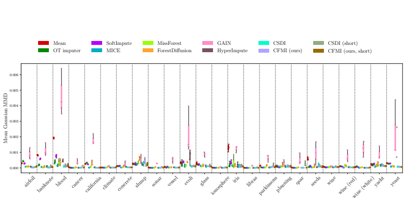
**Figure 7.** Figure 7: Wasserstein-2 results: box-plot of 3 runs. MCAR 25% missingness. [PITH_FULL_IMAGE:figures/full_fig_p037_7.png]

**Figure 8.** Figure 8: Wasserstein-2 results: box-plot of 3 runs. MCAR 50% missingness. [PITH_FULL_IMAGE:figures/full_fig_p038_8.png]

**Figure 9.** Figure 9: Wasserstein-2 results: box-plot of 3 runs. MCAR 75% missingness. [PITH_FULL_IMAGE:figures/full_fig_p038_9.png]

**Figure 10.** Figure 10: Wasserstein-2 results: box-plot of 3 runs. MAR 25% missingness. [PITH_FULL_IMAGE:figures/full_fig_p038_10.png]

**Figure 11.** Figure 11: Average RMSE results: box-plot of 3 runs. MCAR 25% missingness. [PITH_FULL_IMAGE:figures/full_fig_p039_11.png]

**Figure 12.** Figure 12: Average RMSE results: box-plot of 3 runs. MCAR 50% missingness. [PITH_FULL_IMAGE:figures/full_fig_p039_12.png]

**Figure 13.** Figure 13: Average RMSE results: box-plot of 3 runs. MCAR 75% missingness. [PITH_FULL_IMAGE:figures/full_fig_p039_13.png]

**Figure 14.** Figure 14: Average RMSE results: box-plot of 3 runs. MAR 25% missingness. [PITH_FULL_IMAGE:figures/full_fig_p040_14.png]

**Figure 15.** Figure 15: CRPS results: box-plot of 3 runs. MCAR 25% missingness. [PITH_FULL_IMAGE:figures/full_fig_p040_15.png]

**Figure 16.** Figure 16: CRPS results: box-plot of 3 runs. MCAR 50% missingness. [PITH_FULL_IMAGE:figures/full_fig_p040_16.png]

**Figure 17.** Figure 17: CRPS results: box-plot of 3 runs. MCAR 75% missingness. [PITH_FULL_IMAGE:figures/full_fig_p041_17.png]

**Figure 18.** Figure 18: CRPS results: box-plot of 3 runs. MAR 25% missingness. [PITH_FULL_IMAGE:figures/full_fig_p041_18.png]

**Figure 19.** Figure 19: Energy MMD results: box-plot of 3 runs. MCAR 25% missingness. [PITH_FULL_IMAGE:figures/full_fig_p041_19.png]

**Figure 20.** Figure 20: Energy MMD results: box-plot of 3 runs. MCAR 50% missingness. [PITH_FULL_IMAGE:figures/full_fig_p042_20.png]

**Figure 21.** Figure 21: Energy MMD results: box-plot of 3 runs. MCAR 75% missingness. [PITH_FULL_IMAGE:figures/full_fig_p042_21.png]

**Figure 22.** Figure 22: Energy MMD results: box-plot of 3 runs. MAR 25% missingness. [PITH_FULL_IMAGE:figures/full_fig_p042_22.png]

**Figure 23.** Figure 23: Gaussian MMD results: box-plot of 3 runs. MCAR 25% missingness. [PITH_FULL_IMAGE:figures/full_fig_p043_23.png]

**Figure 24.** Figure 24: Gaussian MMD results: box-plot of 3 runs. MCAR 50% missingness. [PITH_FULL_IMAGE:figures/full_fig_p043_24.png]

**Figure 25.** Figure 25: Gaussian MMD results: box-plot of 3 runs. MCAR 75% missingness. [PITH_FULL_IMAGE:figures/full_fig_p043_25.png]

**Figure 26.** Figure 26: Gaussian MMD results: box-plot of 3 runs. MAR 25% missingness. [PITH_FULL_IMAGE:figures/full_fig_p044_26.png]

**Figure 27.** Figure 27: Laplacian MMD results: box-plot of 3 runs. MCAR 25% missingness. [PITH_FULL_IMAGE:figures/full_fig_p044_27.png]

**Figure 28.** Figure 28: Laplacian MMD results: box-plot of 3 runs. MCAR 50% missingness. [PITH_FULL_IMAGE:figures/full_fig_p044_28.png]

**Figure 29.** Figure 29: Laplacian MMD results: box-plot of 3 runs. MCAR 75% missingness. [PITH_FULL_IMAGE:figures/full_fig_p045_29.png]

**Figure 30.** Figure 30: Laplacian MMD results: box-plot of 3 runs. MAR 25% missingness. [PITH_FULL_IMAGE:figures/full_fig_p045_30.png]

**Figure 31.** Figure 31: Classifier 1-AUROC results: box-plot of 3 runs. MCAR 25% missingness. [PITH_FULL_IMAGE:figures/full_fig_p045_31.png]

**Figure 32.** Figure 32: Classifier 1-AUROC results: box-plot of 3 runs. MCAR 50% missingness. [PITH_FULL_IMAGE:figures/full_fig_p046_32.png]

**Figure 33.** Figure 33: Classifier 1-AUROC results: box-plot of 3 runs. MCAR 75% missingness. [PITH_FULL_IMAGE:figures/full_fig_p046_33.png]

**Figure 34.** Figure 34: Classifier 1-AUROC results: box-plot of 3 runs. MAR 25% missingness. [PITH_FULL_IMAGE:figures/full_fig_p046_34.png]

**Figure 35.** Figure 35: Regression CRPS results: box-plot of 3 runs. MCAR 25% missingness. [PITH_FULL_IMAGE:figures/full_fig_p047_35.png]

**Figure 36.** Figure 36: Regression CRPS results: box-plot of 3 runs. MCAR 50% missingness. [PITH_FULL_IMAGE:figures/full_fig_p047_36.png]

**Figure 37.** Figure 37: Regression CRPS results: box-plot of 3 runs. MCAR 75% missingness. [PITH_FULL_IMAGE:figures/full_fig_p047_37.png]

**Figure 38.** Figure 38: Regression CRPS results: box-plot of 3 runs. MAR 25% missingness. [PITH_FULL_IMAGE:figures/full_fig_p048_38.png]

**Figure 39.** Figure 39: Regression parameter percent bias results: box-plot of 3 runs. MCAR 25% missingness. [PITH_FULL_IMAGE:figures/full_fig_p048_39.png]

**Figure 40.** Figure 40: Regression parameter percent bias results: box-plot of 3 runs. MCAR 50% missingness. [PITH_FULL_IMAGE:figures/full_fig_p048_40.png]

**Figure 41.** Figure 41: Regression parameter percent bias results: box-plot of 3 runs. MCAR 75% missingness. [PITH_FULL_IMAGE:figures/full_fig_p049_41.png]

**Figure 42.** Figure 42: Regression parameter percent bias results: box-plot of 3 runs. MAR 25% missingness. [PITH_FULL_IMAGE:figures/full_fig_p049_42.png]

**Figure 43.** Figure 43: Regression parameter 1-CR results: box-plot of 3 runs. MCAR 25% missingness. [PITH_FULL_IMAGE:figures/full_fig_p049_43.png]

**Figure 44.** Figure 44: Regression parameter 1-CR results: box-plot of 3 runs. MCAR 50% missingness. [PITH_FULL_IMAGE:figures/full_fig_p050_44.png]

**Figure 45.** Figure 45: Regression parameter 1-CR results: box-plot of 3 runs. MCAR 75% missingness. [PITH_FULL_IMAGE:figures/full_fig_p050_45.png]

**Figure 46.** Figure 46: Regression parameter 1-CR results: box-plot of 3 runs. MAR 25% missingness. [PITH_FULL_IMAGE:figures/full_fig_p050_46.png]

**Figure 47.** Figure 47: Regression parameter AW results: box-plot of 3 runs. MCAR 25% missingness. [PITH_FULL_IMAGE:figures/full_fig_p051_47.png]

**Figure 48.** Figure 48: Regression parameter AW results: box-plot of 3 runs. MCAR 50% missingness. [PITH_FULL_IMAGE:figures/full_fig_p051_48.png]

**Figure 49.** Figure 49: Regression parameter AW results: box-plot of 3 runs. MCAR 75% missingness. [PITH_FULL_IMAGE:figures/full_fig_p051_49.png]

**Figure 50.** Figure 50: Regression parameter AW results: box-plot of 3 runs. MAR 25% missingness. [PITH_FULL_IMAGE:figures/full_fig_p052_50.png]

**Figure 51.** Figure 51: Wasserstein-2 results: average relative distance (blue means row method outperforms the column method). MCAR 25% missingness. OT imputer SoftImpute MICE MissForest ForestDiffusion GAIN HyperImpute CSDI CFMI (ours) CSDI (short) CFMI (ours, short) OT imputer SoftImpute …

**Figure 53.** Figure 53: Wasserstein-2 results: average relative distance (blue means row method outperforms the column method). MCAR 75% missingness. OT imputer SoftImpute MICE MissForest ForestDiffusion GAIN HyperImpute CSDI CFMI (ours) CSDI (short) CFMI (ours, short) OT imputer SoftImpute …

**Figure 55.** Figure 55: Average RMSE results: average relative distance (blue means row method outperforms the column method). MCAR 25% missingness. OT imputer SoftImpute MICE MissForest ForestDiffusion GAIN HyperImpute CSDI CFMI (ours) CSDI (short) CFMI (ours, short) OT imputer SoftImpute M…

**Figure 57.** Figure 57: Average RMSE results: average relative distance (blue means row method outperforms the column method). MCAR 75% missingness. OT imputer SoftImpute MICE MissForest ForestDiffusion GAIN HyperImpute CSDI CFMI (ours) CSDI (short) CFMI (ours, short) OT imputer SoftImpute M…

**Figure 59.** Figure 59: CRPS results: average relative distance (blue means row method outperforms the column method). MCAR 25% missingness. OT imputer SoftImpute MICE MissForest ForestDiffusion GAIN HyperImpute CSDI CFMI (ours) CSDI (short) CFMI (ours, short) OT imputer SoftImpute MICE Miss…

**Figure 61.** Figure 61: CRPS results: average relative distance (blue means row method outperforms the column method). MCAR 75% missingness. OT imputer SoftImpute MICE MissForest ForestDiffusion GAIN HyperImpute CSDI CFMI (ours) CSDI (short) CFMI (ours, short) OT imputer SoftImpute MICE Miss…

**Figure 63.** Figure 63: Energy MMD results: average relative distance (blue means row method outperforms the column method). MCAR 25% missingness. OT imputer SoftImpute MICE MissForest ForestDiffusion GAIN HyperImpute CSDI CFMI (ours) CSDI (short) CFMI (ours, short) OT imputer SoftImpute MIC…

**Figure 65.** Figure 65: Energy MMD results: average relative distance (blue means row method outperforms the column method). MCAR 75% missingness. OT imputer SoftImpute MICE MissForest ForestDiffusion GAIN HyperImpute CSDI CFMI (ours) CSDI (short) CFMI (ours, short) OT imputer SoftImpute MIC…

**Figure 67.** Figure 67: Gaussian MMD results: average relative distance (blue means row method outperforms the column method). MCAR 25% missingness. OT imputer SoftImpute MICE MissForest ForestDiffusion GAIN HyperImpute CSDI CFMI (ours) CSDI (short) CFMI (ours, short) OT imputer SoftImpute M…

**Figure 69.** Figure 69: Gaussian MMD results: average relative distance (blue means row method outperforms the column method). MCAR 75% missingness. OT imputer SoftImpute MICE MissForest ForestDiffusion GAIN HyperImpute CSDI CFMI (ours) CSDI (short) CFMI (ours, short) OT imputer SoftImpute M…

**Figure 71.** Figure 71: Laplacian MMD results: average relative distance (blue means row method outperforms the column method). MCAR 25% missingness. OT imputer SoftImpute MICE MissForest ForestDiffusion GAIN HyperImpute CSDI CFMI (ours) CSDI (short) CFMI (ours, short) OT imputer SoftImpute …

**Figure 73.** Figure 73: Laplacian MMD results: average relative distance (blue means row method outperforms the column method). MCAR 75% missingness. OT imputer SoftImpute MICE MissForest ForestDiffusion GAIN HyperImpute CSDI CFMI (ours) CSDI (short) CFMI (ours, short) OT imputer SoftImpute …

**Figure 75.** Figure 75: Classifier 1-AUROC results: average rel [PITH_FULL_IMAGE:figures/full_fig_p059_75.png]

**Figure 77.** Figure 77: Classifier 1-AUROC results: average rel [PITH_FULL_IMAGE:figures/full_fig_p059_77.png]

**Figure 79.** Figure 79: Regression CRPS results: average relative distance (blue means row method outperforms the column method). MCAR 25% missingness. OT imputer SoftImpute MICE MissForest ForestDiffusion GAIN HyperImpute CSDI CFMI (ours) CSDI (short) CFMI (ours, short) OT imputer SoftImpu…

**Figure 81.** Figure 81: Regression CRPS results: average relative distance (blue means row method outperforms the column method). MCAR 75% missingness. OT imputer SoftImpute MICE MissForest ForestDiffusion GAIN HyperImpute CSDI CFMI (ours) CSDI (short) CFMI (ours, short) OT imputer SoftImpu…

**Figure 83.** Figure 83: Regression parameter percent bias results: average relative distance (blue means row method outperforms the column method). MCAR 25% missingness. OT imputer SoftImpute MICE MissForest ForestDiffusion GAIN HyperImpute CSDI CFMI (ours) CSDI (short) CFMI (ours, short) O…

**Figure 85.** Figure 85: Regression parameter percent bias results: average relative distance (blue means row method outperforms the column method). MCAR 75% missingness. OT imputer SoftImpute MICE MissForest ForestDiffusion GAIN HyperImpute CSDI CFMI (ours) CSDI (short) CFMI (ours, short) O…

**Figure 87.** Figure 87: Regression parameter 1-CR results: average relative distance (blue means row method outperforms the column method). MCAR 25% missingness. OT imputer SoftImpute MICE MissForest ForestDiffusion GAIN HyperImpute CSDI CFMI (ours) CSDI (short) CFMI (ours, short) OT impu…

**Figure 89.** Figure 89: Regression parameter 1-CR results: average relative distance (blue means row method outperforms the column method). MCAR 75% missingness. OT imputer SoftImpute MICE MissForest ForestDiffusion GAIN HyperImpute CSDI CFMI (ours) CSDI (short) CFMI (ours, short) OT impu…

**Figure 91.** Figure 91: Regression parameter AW results: average relative distance (blue means row method outperforms the column method). MCAR 25% missingness. OT imputer SoftImpute MICE MissForest ForestDiffusion GAIN HyperImpute CSDI CFMI (ours) CSDI (short) CFMI (ours, short) OT impute…

**Figure 93.** Figure 93: Regression parameter AW results: average relative distance (blue means row method outperforms the column method). MCAR 75% missingness. OT imputer SoftImpute MICE MissForest ForestDiffusion GAIN HyperImpute CSDI CFMI (ours) CSDI (short) CFMI (ours, short) OT impute…

**Figure 95.** Figure 95: Average rank on Wasserstein-2 over all data sets versus missingness fraction. MCAR missingness. [PITH_FULL_IMAGE:figures/full_fig_p065_95.png]

**Figure 96.** Figure 96: Average rank on average RMSE over all data sets versus missingness fraction. MCAR missingness. [PITH_FULL_IMAGE:figures/full_fig_p065_96.png]

**Figure 97.** Figure 97: Average rank on CRPS over all data sets versus missingness fraction. MCAR missingness. [PITH_FULL_IMAGE:figures/full_fig_p066_97.png]

**Figure 98.** Figure 98: Average rank on energy MMD over all data sets versus missingness fraction. MCAR missingness. [PITH_FULL_IMAGE:figures/full_fig_p066_98.png]

**Figure 99.** Figure 99: Average rank on Gaussian MMD over all data sets versus missingness fraction. MCAR missing [PITH_FULL_IMAGE:figures/full_fig_p066_99.png]

**Figure 100.** Figure 100: Average rank on Laplacian MMD over all data sets versus missingness fraction. MCAR miss [PITH_FULL_IMAGE:figures/full_fig_p067_100.png]

**Figure 101.** Figure 101: Average rank on classifier 1-AUROC over all data sets versus missingness fraction. MCAR [PITH_FULL_IMAGE:figures/full_fig_p067_101.png]

**Figure 102.** Figure 102: Average rank on regression CRPS over all data sets versus missingness fraction. MCAR miss [PITH_FULL_IMAGE:figures/full_fig_p068_102.png]

**Figure 103.** Figure 103: Average rank on regression parameter PB over all data sets versus missingness fraction. MCAR [PITH_FULL_IMAGE:figures/full_fig_p068_103.png]

**Figure 104.** Figure 104: Average rank on regression parameter 1-CR over all data sets versus missingness fraction. MCAR [PITH_FULL_IMAGE:figures/full_fig_p069_104.png]

**Figure 105.** Figure 105: Average rank on regression parameter AW over all data sets versus missingness fraction. MCAR [PITH_FULL_IMAGE:figures/full_fig_p069_105.png]

**Figure 106.** Figure 106: Wasserstein-2 metric vs number of training steps. MCAR 25% missingness. [PITH_FULL_IMAGE:figures/full_fig_p070_106.png]

**Figure 107.** Figure 107: Wasserstein-2 metric vs number of training steps. MAR 25% missingness. [PITH_FULL_IMAGE:figures/full_fig_p071_107.png]

**Figure 108.** Figure 108: Average RMSE metric vs number of training steps. MCAR 25% missingness. [PITH_FULL_IMAGE:figures/full_fig_p072_108.png]

**Figure 109.** Figure 109: Average RMSE metric vs number of training steps. MAR 25% missingness. [PITH_FULL_IMAGE:figures/full_fig_p073_109.png]

**Figure 110.** Figure 110: CRPS metric vs number of training steps. MCAR 25% missingness. [PITH_FULL_IMAGE:figures/full_fig_p074_110.png]

**Figure 111.** Figure 111: CRPS metric vs number of training steps. MAR 25% missingness. [PITH_FULL_IMAGE:figures/full_fig_p075_111.png]

**Figure 112.** Figure 112: Energy MMD metric vs number of training steps. MCAR 25% missingness. [PITH_FULL_IMAGE:figures/full_fig_p076_112.png]

**Figure 113.** Figure 113: Energy MMC metric vs number of training steps. MAR 25% missingness. [PITH_FULL_IMAGE:figures/full_fig_p077_113.png]

**Figure 114.** Figure 114: Gaussian MMD metric vs number of training steps. MCAR 25% missingness. [PITH_FULL_IMAGE:figures/full_fig_p078_114.png]

**Figure 115.** Figure 115: Gaussian MMC metrics vs number of training steps. MAR 25% missingness. [PITH_FULL_IMAGE:figures/full_fig_p079_115.png]

**Figure 116.** Figure 116: Laplacian MMD metric vs number of training steps. MCAR 25% missingness. [PITH_FULL_IMAGE:figures/full_fig_p080_116.png]

**Figure 117.** Figure 117: Laplacian MMC metric vs number of training steps. MAR 25% missingness. [PITH_FULL_IMAGE:figures/full_fig_p081_117.png]

**Figure 118.** Figure 118: Classifier 1-AUROC metric vs number of training steps. MCAR 25% missingness. [PITH_FULL_IMAGE:figures/full_fig_p082_118.png]

**Figure 119.** Figure 119: Classifier 1-AUROC metric vs number of training steps. MAR 25% missingness. [PITH_FULL_IMAGE:figures/full_fig_p083_119.png]

**Figure 120.** Figure 120: Regression CRPS metric vs number of training steps. MCAR 25% missingness. [PITH_FULL_IMAGE:figures/full_fig_p084_120.png]

**Figure 121.** Figure 121: Regression CRPS metric vs number of training steps. MAR 25% missingness. [PITH_FULL_IMAGE:figures/full_fig_p085_121.png]

**Figure 122.** Figure 122: Regression parameter PB metric vs number of training steps. MCAR 25% missingness. [PITH_FULL_IMAGE:figures/full_fig_p086_122.png]

**Figure 123.** Figure 123: Regression parameter PB metric vs number of training steps. MAR 25% missingness. [PITH_FULL_IMAGE:figures/full_fig_p087_123.png]

**Figure 124.** Figure 124: Regression parameter 1-CR metric vs number of training steps. MCAR 25% missingness. [PITH_FULL_IMAGE:figures/full_fig_p088_124.png]

**Figure 125.** Figure 125: Regression parameter 1-CR metric vs number of training steps. MAR 25% missingness. [PITH_FULL_IMAGE:figures/full_fig_p089_125.png]

**Figure 126.** Figure 126: Regression parameter AW metric vs number of training steps. MCAR 25% missingness. [PITH_FULL_IMAGE:figures/full_fig_p090_126.png]

**Figure 127.** Figure 127: Regression parameter AW metric vs number of training steps. MAR 25% missingness. [PITH_FULL_IMAGE:figures/full_fig_p091_127.png]

**Figure 128.** Figure 128: CRPS versus number of training epochs. 101 102 epochs 3 × 10−1 4 × 10−1 6 × 10−1 Normalised CRPS 10% missing CSDI CFMI (ours) 101 102 epochs 4 × 10−1 5 × 10−1 6 × 10−1 7 × 10−1 PhysioNet 50% missing 101 102 epochs 5 × 10−1 6 × 10−1 7 × 10−1 8 × 10−1 90% missing 101 1…

**Figure 129.** Figure 129: Magnitude-normalised CRPS versus number of training epochs. [PITH_FULL_IMAGE:figures/full_fig_p093_129.png]

**Figure 130.** Figure 130: MAE versus number of training epochs. 101 102 epochs 100 6 × 10−1 2 × 100 RMSE 10% missing CSDI CFMI (ours) 101 102 epochs 100 6 × 10−1 PhysioNet 50% missing 101 102 epochs 100 8 × 10−1 9 × 10−1 90% missing 101 102 epochs 2 × 101 3 × 101 4 × 101 PM2.5 [PITH_FULL_IMA…

**Figure 131.** Figure 131: RMSE versus number of training epochs. 94 [PITH_FULL_IMAGE:figures/full_fig_p094_131.png]

Discussion (0). Continue with ORCID to comment.

Forward citations

Cited by 2 Pith papers

Reviewed papers in the Pith corpus that reference this work. Sorted by Pith novelty score. Full citation record

Neural Conditional Simulation for Complex Spatial Processes
stat.ME 2025-08 conditional novelty 6.0 of 10

Neural conditional simulation trains a masked diffusion model on unconditional spatial field samples to draw from predictive distributions, demonstrated on Gaussian and Brown–Resnick processes.
Flow Matching with Missing Data
cs.LG 2026-07 conditional novelty 5.0 of 10

Resampling missing coordinates and averaging the flow-matching loss reproduces the complete-data objective exactly under MCAR with oracle completions; one completion per example is optimal for a fixed budget.

Reference graph

Works this paper leans on

73 extracted references · 55 canonical work pages · cited by 2 Pith papers

[1]

and Forina, M

Aeberhard, S. and Forina, M. Wine, 1992

work page 1992
[2]

S., Boffi, N

Albergo, M. S., Boffi, N. M., and Vanden-Eijnden , E. Stochastic Interpolants : A Unifying Framework for Flows and Diffusions , November 2023

work page 2023
[3]

Planning Relax , 2004

Bhatt, R. Planning Relax , 2004

work page 2004
[4]

V., Chai, K., and Williams, C

Bonilla, E. V., Chai, K., and Williams, C. K. I. Multi-task Gaussian Process Prediction . In Advances in Neural Information Processing Systems ( NeurIPS ) , 2007

work page 2007
[5]

Airfoil Self-Noise , 1989

Brooks, T., Pope, D., and Michael Marcolini . Airfoil Self-Noise , 1989

work page 1989
[6]

BRITS : Bidirectional Recurrent Imputation for Time Series

Cao, W., Wang, D., Li, J., Zhou, H., Li, L., and Li, Y. BRITS : Bidirectional Recurrent Imputation for Time Series . In Neural Information Processing Systems ( NeurIPS ) , 2018

work page 2018
[7]

Seeds, 2010

Charytanowicz, M., Niewczas, J., Kulczycki, P., Kowalski, P., and Lukasik, S. Seeds, 2010

work page 2010
[8]

Chen, R. T. Q., Rubanova, Y., Bettencourt, J., and Duvenaud, D. Neural Ordinary Differential Equations . In International Series in Operations Research and Management Science , 2019

work page 2019

Show all 73 references

[9]

RDIS : Random Drop Imputation with Self-Training for Incomplete Time Series Data

Choi, T.-M., Kang, J.-S., and Kim, J.-H. RDIS : Random Drop Imputation with Self-Training for Incomplete Time Series Data . In AAAI Conference on Artificial Intelligence , 2023. doi:10.1109/ACCESS.2023.3315343

2023
[10]

Wine Quality , 2009

Cortez, P., Cerdeira, A., Almeida, F., Matos, T., and Reis, J. Wine Quality , 2009

2009
[11]

R., Macke, J

Dax, M., Wildberger, J., Buchholz, S., Green, S. R., Macke, J. H., and Sch \"o lkopf, B. Flow Matching for Scalable Simulation-Based Inference . In Neural Information Processing Systems ( NeurIPS ) , October 2023. doi:10.48550/arXiv.2305.17161

2023 doi arXiv
[12]

P., Laird, N

Dempster, A. P., Laird, N. M., and Rubin, D. B. Maximum Likelihood from Incomplete Data Via the EM Algorithm . Journal of the Royal Statistical Society: Series B (Methodological), 39 0 (1): 0 1--22, 1977. doi:10.1111/j.2517-6161.1977.tb01600.x

1977
[13]

Connectionist Bench ( Vowel Recognition - Deterding Data ), 1988

Deterding, D., Niranjan, M., and Robinson, T. Connectionist Bench ( Vowel Recognition - Deterding Data ), 1988

1988
[14]

Libras Movement , 2009

Dias, D., Peres, S., and Bscaro, H. Libras Movement , 2009

2009
[15]

A Universal Marginalizer for Amortized Inference in Generative Models

Douglas, L., Zarov, I., Gourgoulias, K., Lucas, C., Hart, C., Baker, A., Sahani, M., Perov, Y., and Johri, S. A Universal Marginalizer for Amortized Inference in Generative Models . In Workshop on Advances in Approximate Bayesian Inference ( NeurIPS ) , November 2017

2017
[16]

and Graff, C

Dua, D. and Graff, C. UCI Machine Learning Repository , 2017

2017
[17]

Interpolating between Optimal Transport and MMD using Sinkhorn Divergences

Feydy, J., S \'e journ \'e , T., Vialard, F.-X., Amari, S.-i., Trouv \'e , A., and Peyr \'e , G. Interpolating between Optimal Transport and MMD using Sinkhorn Divergences . In International Conference on Artificial Intelligence and Statistics ( AISTATS ) , 2019. doi:10.48550/...

2019 doi arXiv
[18]

Fisher, R. A. Iris, 1936

1936
[19]

Z., Boisbunon, A., Chambon, S., Chapel, L., Corenflos, A., Fatras, K., Fournier, N., Gautheron, L., Gayraud, N

Flamary, R., Courty, N., Gramfort, A., Alaya, M. Z., Boisbunon, A., Chambon, S., Chapel, L., Corenflos, A., Fatras, K., Fournier, N., Gautheron, L., Gayraud, N. T. H., Janati, H., Rakotomamonjy, A., Redko, I., Rolet, A., Schutz, A., Seguy, V., Sutherland, D. J., Tavenard, R., ...

2021
[20]

GP-VAE : Deep Probabilistic Time Series Imputation

Fortuin, V., Baranchuk, D., R \"a tsch, G., and Mandt, S. GP-VAE : Deep Probabilistic Time Series Imputation . In International Conference on Artificial Intelligence and Statistics ( AISTATS ) , February 2020. doi:10.48550/arXiv.1907.04155

2020 doi arXiv
[21]

Gat, I., Remez, T., Shaul, N., Kreuk, F., Chen, R. T. Q., Synnaeve, G., Adi, Y., and Lipman, Y. Discrete Flow Matching . In Neural Information Processing Systems ( NeurIPS ) , November 2024. doi:10.48550/arXiv.2407.15595

2024 doi arXiv
[22]

Glass Identification , 1987

German, B. Glass Identification , 1987

1987
[23]

Yacht Hydrodynamics , 1981

Gerritsma, J., Onnink, R., and Versluis, A. Yacht Hydrodynamics , 1981

1981
[24]

M., Rasch, M

Gretton, A., Borgwardt, K. M., Rasch, M. J., Sch \"o lkopf, B., and Smola, A. A Kernel Two-Sample Test . Journal of Machine Learning Research, 13 0 (25): 0 723--773, 2012. ISSN 1533-7928

2012
[25]

D., and Zadeh, R

Hastie, T., Mazumder, R., Lee, J. D., and Zadeh, R. Matrix Completion and Low-Rank SVD via Fast Alternating Least Squares . Journal of Machine Learning Research, 16 0 (104): 0 3367--3402, 2015. ISSN 1533-7928

2015
[26]

Denoising Diffusion Probabilistic Models

Ho, J., Jain, A., and Abbeel, P. Denoising Diffusion Probabilistic Models . In Neural Information Processing Systems ( NeurIPS ) , December 2020. doi:10.48550/arXiv.2006.11239

2020 doi arXiv
[27]

Variational Autoencoder with Arbitrary Conditioning

Ivanov, O., Figurnov, M., and Vetrov, D. Variational Autoencoder with Arbitrary Conditioning . In arXiv Pre-Print , 2019

2019
[28]

C., Liu, T., Curth, A., and van der Schaar, M

Jarrett, D., Cebere, B. C., Liu, T., Curth, A., and van der Schaar, M. HyperImpute : Generalized Iterative Imputation with Automatic Model Selection . In International Conference on Machine Learning ( ICML ) , June 2022

2022
[29]

Generating and Imputing Tabular Data via Diffusion and Flow-based Gradient-Boosted Trees

Jolicoeur-Martineau , A., Fatras, K., and Kachman, T. Generating and Imputing Tabular Data via Diffusion and Flow-based Gradient-Boosted Trees . In International Conference on Artificial Intelligence and Statistics ( AISTATS ) , February 2024. doi:10.48550/arXiv.2309.09968

2024 doi arXiv
[30]

Kingma, D. P. and Ba, J. L. Adam: A Method for Stochastic Optimization . In International Conference on Learning Representations ( ICLR ) , December 2014

2014
[31]

DiffWave : A Versatile Diffusion Model for Audio Synthesis

Kong, Z., Ping, W., Huang, J., Zhao, K., and Catanzaro, B. DiffWave : A Versatile Diffusion Model for Audio Synthesis . In International Conference on Learning Representations ( ICLR ) , March 2021. doi:10.48550/arXiv.2009.09761

2021 doi arXiv
[32]

Li, Y., Akbar, S., and Oliva, J. B. Flow Models for Arbitrary Conditional Likelihoods . In International Conference on Machine Learning ( ICML ) , 2020

2020
[33]

Lipman, Y., Chen, R. T. Q., Ben-Hamu , H., Nickel, M., and Le, M. Flow Matching for Generative Modeling . In International Conference on Learning Representations ( ICLR ) , February 2023. doi:10.48550/arXiv.2210.02747

2023 doi arXiv
[34]

Parkinsons, 2007

Little, M. Parkinsons, 2007

2007
[35]

Little, R. J. A. and Rubin, D. B. Statistical Analysis with Missing Data : Third Edition . Wiley Series in Probability and Statistics. Wiley, Hoboken, NJ, 3rd edition edition, 2020. ISBN 978-1-119-48226-0

2020
[36]

Banknote Authentication , 2012

Lohweg, V. Banknote Authentication , 2012

2012
[37]

and Hutter, F

Loshchilov, I. and Hutter, F. Decoupled Weight Decay Regularization . In International Conference on Learning Representations ( ICLR ) , November 2017

2017
[38]

Climate Model Simulation Crashes , 2013

Lucas, D., Klein, R., Tannahill, J., Ivanova, D., Brandon, S., Domyancic, D., and Zhang, Y. Climate Model Simulation Crashes , 2013

2013
[39]

RePaint : Inpainting using Denoising Diffusion Probabilistic Models , August 2022

Lugmayr, A., Danelljan, M., Romero, A., Yu, F., Timofte, R., and Van Gool, L. RePaint : Inpainting using Denoising Diffusion Probabilistic Models , August 2022

2022
[40]

QSAR biodegradation, 2013

Mansouri, K., Ringsted, T., Ballabio, D., Todeschini, R., and Consonni, V. QSAR biodegradation, 2013

2013
[41]

Matheson, J. E. and Winkler, R. L. Scoring Rules for Continuous Probability Distributions . Management Science, 22 0 (10): 0 1087--1096, 1976. ISSN 0025-1909

1976
[42]

and Frellsen, J

Mattei, P.-A. and Frellsen, J. MIWAE : Deep Generative Modelling and Imputation of Incomplete Data Sets . In International Conference on Machine Learning ( ICML ) , 2019

2019
[43]

Generative Semi-supervised Learning for Multivariate Time Series Imputation

Miao, X., Wu, Y., Wang, J., Gao, Y., Mao, X., and Yin, J. Generative Semi-supervised Learning for Multivariate Time Series Imputation . In AAAI Conference on Artificial Intelligence , May 2021. doi:10.1609/aaai.v35i10.17086

2021 doi
[44]

W., Jun, E., and Suk, H.-I

Mulyadi, A. W., Jun, E., and Suk, H.-I. Uncertainty- Aware Variational-Recurrent Imputation Network for Clinical Time Series . IEEE Transactions on Cybernetics, 52 0 (9), November 2020. doi:10.48550/arXiv.2003.00662

2020 doi arXiv
[45]

Murphy, K. P. Probabilistic Machine Learning : An Introduction . MIT Press, 2021

2021
[46]

Missing Data Imputation using Optimal Transport

Muzellec, B., Josse, J., Boyer, C., and Cuturi, M. Missing Data Imputation using Optimal Transport . In International Conference on Machine Learning ( ICML ) , 2020

2020
[47]

Yeast, 1991

Nakai, K. Yeast, 1991

1991
[48]

Ecoli, 1996

Nakai, K. Ecoli, 1996

1996
[49]

Pace, R. K. and Barry, R. Sparse spatial autoregressions. Statistics & Probability Letters, 33 0 (3): 0 291--297, May 1997. ISSN 0167-7152. doi:10.1016/S0167-7152(96)00140-X

1997 doi
[50]

PyTorch : An Imperative Style , High-Performance Deep Learning Library

Paszke, A., Gross, S., Massa, F., Lerer, A., Bradbury, J., Chanan, G., Killeen, T., Lin, Z., Gimelshein, N., Antiga, L., Desmaison, A., K \"o pf, A., Yang, E., DeVito, Z., Raison, M., Tejani, A., Chilamkurthy, S., Steiner, B., Fang, L., Bai, J., and Chintala, S. PyTorch : An I...

2019 doi arXiv
[51]

J., Dubourg, V., Vanderplas, J., Passos, A., Cournapeau, D., Brucher, M., Perrot, M., and Duchesnay, \'E

Pedregosa, F., Varoquaux, G., Gramfort, A., Michel, V., Thirion, B., Grisel, O., Blondel, M., Prettenhofer, P., Weiss, R. J., Dubourg, V., Vanderplas, J., Passos, A., Cournapeau, D., Brucher, M., Perrot, M., and Duchesnay, \'E . Scikit-learn: Machine Learning in Python . Journ...

2011
[52]

Rubin, D. B. Multiple Imputation for Nonresponse in Surveys . John Wiley & Sons, New York, 1987. ISBN 0-471-08705-X. doi:10.2307/3172772

1987 doi
[53]

M., Lugtig, P., and Vink, G

Schouten, R. M., Lugtig, P., and Vink, G. Generating missing values for simulation purposes: A multivariate amputation procedure. Journal of Statistical Computation and Simulation, 0 0 (0): 0 1--22, 2018. ISSN 0094-9655. doi:10.1080/00949655.2018.1491577

2018
[54]

and Gorman, R

Sejnowski, T. and Gorman, R. Connectionist Bench ( Sonar , Mines vs. Rocks ), 1988

1988
[55]

Ionosphere, 1989

Sigillito, V., Wing, S., Hutton, L., and Baker, K. Ionosphere, 1989

1989
[56]

J., Celi, L

Silva, I., Moody, G., Scott, D. J., Celi, L. A., and Mark, R. G. Predicting In-Hospital Mortality of ICU Patients : The PhysioNet / Computing in Cardiology Challenge 2012. Computing in cardiology, 39: 0 245--248, 2012

2012
[57]

Simkus, V., Rhodes, B., and Gutmann, M. U. Variational Gibbs Inference for Statistical Model Estimation from Incomplete Data . Journal of Machine Learning Research, 24 0 (196): 0 1--72, 2023. ISSN 1533-7928

2023
[58]

A., Maheswaranathan, N., and Ganguli, S

Sohl-Dickstein , J., Weiss, E. A., Maheswaranathan, N., and Ganguli, S. Deep Unsupervised Learning using Nonequilibrium Thermodynamics . In International Conference on Machine Learning ( ICML ) , November 2015. doi:10.48550/arXiv.1503.03585

2015 doi arXiv
[59]

Denoising Diffusion Implicit Models

Song, J., Meng, C., and Ermon, S. Denoising Diffusion Implicit Models . In International Conference on Learning Representations ( ICLR ) , October 2022. doi:10.48550/arXiv.2010.02502

2022 doi arXiv
[60]

Stekhoven, D. J. and B \"u hlmann, P. MissForest - nonparametric missing value imputation for mixed-type data. Bioinformatics, 28 0 (1): 0 112--118, January 2012. ISSN 1367-4803, 1460-2059. doi:10.1093/bioinformatics/btr597

2012 doi
[61]

Strauss, R. R. and Oliva, J. B. Arbitrary Conditional Distributions with Energy . In Neural Information Processing Systems ( NeurIPS ) , October 2021. doi:10.48550/arXiv.2102.04426

2021 doi arXiv
[62]

GLIMA : Global and Local Time Series Imputation with Multi-directional Attention Learning

Suo, Q., Zhong, W., Xun, G., Sun, J., Chen, C., and Zhang, A. GLIMA : Global and Local Time Series Imputation with Multi-directional Attention Learning . In IEEE International Conference on Big Data ( Big Data ) , pp.\ 798--807, December 2020. doi:10.1109/BigData50022.2020.9378408

2020
[63]

CSDI : Conditional Score-based Diffusion Models for Probabilistic Time Series Imputation

Tashiro, Y., Song, J., Song, Y., and Ermon, S. CSDI : Conditional Score-based Diffusion Models for Probabilistic Time Series Imputation . In Neural Information Processing Systems ( NeurIPS ) , October 2021. doi:10.48550/arXiv.2107.03502

2021 doi arXiv
[64]

Improving and generalizing flow-based generative models with minibatch optimal transport

Tong, A., Malkin, N., Huguet, G., Zhang, Y., Rector-Brooks , J., Fatras, K., Wolf, G., and Bengio, Y. Improving and generalizing flow-based generative models with minibatch optimal transport. Transactions on Machine Learning Research, October 2023. doi:10.48550/arXiv.2302.00482

2023 doi arXiv
[65]

Flexible Imputation of Missing Data

van Buuren , S. Flexible Imputation of Missing Data . CRC Press LLC, 2 edition, 2018. ISBN 978-1-138-58831-8

2018
[66]

and Oudshoorn, C

van Buuren , S. and Oudshoorn, C. G. M. Multivariate Imputation by Chained Equations . Technical report, TNO Prevention and Health , 2000

2000
[67]

J., Strathmann, H., and Gretton, A

Wenliang, L., Sutherland, D. J., Strathmann, H., and Gretton, A. Learning deep kernels for exponential family densities. In International Conference on Machine Learning ( ICML ) , 2019. doi:10.48550/arXiv.1811.08357

2019 doi arXiv
[68]

Breast Cancer Wisconsin ( Diagnostic ), 1993

Wolberg, W., Mangasarian, O., Street, N., and Street, W. Breast Cancer Wisconsin ( Diagnostic ), 1993

1993
[69]

Concrete Compressive Strength , 1998

Yeh, I.-C. Concrete Compressive Strength , 1998

1998
[70]

Concrete Slump Test , 2007

Yeh, I.-C. Concrete Slump Test , 2007

2007
[71]

Blood Transfusion Service Center , 2008

Yeh, I.-C. Blood Transfusion Service Center , 2008

2008
[72]

ST-MVL : Filling Missing Values in Geo-Sensory Time Series Data

Yi, X., Zheng, Y., Zhang, J., and Li, T. ST-MVL : Filling Missing Values in Geo-Sensory Time Series Data . In International Joint Conference on Artificial Intelligence ( IJCAI ) , 2016

2016
[73]

GAIN : Missing Data Imputation using Generative Adversarial Nets

Yoon, J., Jordon, J., and van der Schaar , M. GAIN : Missing Data Imputation using Generative Adversarial Nets . In International Conference of Machine Learning ( ICML ) , June 2018

2018

Pith tools

Reviewed August 7, 2026 · model on record in the stance chip above.

[1] [1]

and Forina, M

Aeberhard, S. and Forina, M. Wine, 1992

work page 1992

[2] [2]

S., Boffi, N

Albergo, M. S., Boffi, N. M., and Vanden-Eijnden , E. Stochastic Interpolants : A Unifying Framework for Flows and Diffusions , November 2023

work page 2023

[3] [3]

Planning Relax , 2004

Bhatt, R. Planning Relax , 2004

work page 2004

[4] [4]

V., Chai, K., and Williams, C

Bonilla, E. V., Chai, K., and Williams, C. K. I. Multi-task Gaussian Process Prediction . In Advances in Neural Information Processing Systems ( NeurIPS ) , 2007

work page 2007

[5] [5]

Airfoil Self-Noise , 1989

Brooks, T., Pope, D., and Michael Marcolini . Airfoil Self-Noise , 1989

work page 1989

[6] [6]

BRITS : Bidirectional Recurrent Imputation for Time Series

Cao, W., Wang, D., Li, J., Zhou, H., Li, L., and Li, Y. BRITS : Bidirectional Recurrent Imputation for Time Series . In Neural Information Processing Systems ( NeurIPS ) , 2018

work page 2018

[7] [7]

Seeds, 2010

Charytanowicz, M., Niewczas, J., Kulczycki, P., Kowalski, P., and Lukasik, S. Seeds, 2010

work page 2010

[8] [8]

Chen, R. T. Q., Rubanova, Y., Bettencourt, J., and Duvenaud, D. Neural Ordinary Differential Equations . In International Series in Operations Research and Management Science , 2019

work page 2019