REVIEW 3 major objections 6 minor 46 references
Neural Functions for Learning Periodic Signal
T0 review · 3 major / 6 minor · reviewed 2026-08-07 · deepseek-v4-flash
Pith's one-line read NeRT, an implicit neural representation built from a learnable Fourier feature network times a scale factor, extrapolates periodic signals accurately where standard INRs fail.
desk verdict NeRT is a clean periodic/scale INR factorization that performs well in the reported experiments, but the extrapolation claim is partly built into the calendar coordinate encoding and the theory is asserted rather than derived. read the letter →
The pith
A machine-rendered reading of the paper's core claim, the machinery that carries it, and where it could break.
The reading
What carries the argument
The load-bearing object is the learnable Fourier feature mapping $\psi_F(c^t_i;\theta_F) = \{A_m \odot \sin(\omega_m c^t_{i,m} + \delta_m) + B_m\}_{m=1}^{D_{c_t}}$, where frequencies $\omega_m$ are sampled from a uniform range and amplitudes, phases, and biases are learned. This mapping is what lets the periodic decoder see the temporal structure, and its bounded amplitude keeps the periodic factor in a fixed range; combining it with the unbounded scale decoder $\phi_s$ gives the trend. The second piece is the temporal-coordinate rescaling to a closed finite interval, so future timestamps correspond to in-domain coordinates and extrapolation behaves like interpolation.
What would settle it
Train NeRT on a strictly periodic signal whose period is longer than the encoded interval, so the map $[S_{\min}, S_{\max}]$ cannot wrap one full cycle; if extrapolation error stays low, the bounded-Fourier explanation is incomplete, and if error jumps, the coordinate-wrapping premise is the load-bearing part.
Extended reading notes
Core claim
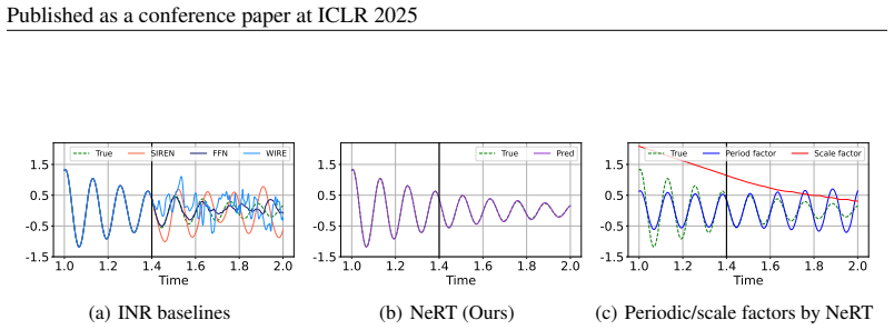
The central claim is that the failure of existing INRs at extrapolation is not inherent but comes from their monolithic treatment of coordinates: a network that explicitly separates periodicity from scale can continue a periodic signal correctly. NeRT computes the signal as $\hat{x} = \hat{x}_{\mathrm{period}} \times \hat{x}_{\mathrm{scale}}$, with $\hat{x}_{\mathrm{period}} \in [-1,1]$ produced by a sinusoidal decoder fed by a learnable Fourier feature map $\psi_F$, and $\hat{x}_{\mathrm{scale}} \in \mathbb{R}$ produced by a separate decoder. The learnable Fourier map has bounded outputs through its amplitude term, so by the extreme value theorem the periodic branch stays confined, and the temporal coordinate is rescaled onto a closed interval $[S_{\min}, S_{\max}]$; the authors argue that extrapolation in original time is then effectively interpolation in the learned coordinate. Empirically, in the atmospheric temperature benchmark they state that only NeRT successfully captures periodicity and predicts the test interval, and in Table 1 NeRT reports the lowest MSE on both interpolation and extrapolation of periodic time series.
Load-bearing premise
The temporal coordinate is always rescaled into a fixed closed interval, so future times are treated as points inside the training domain; this only works when the signal truly repeats with the period that the learned mapping has captured.
Editorial extensions
If this is right
- A single NeRT model trained once can be queried at any future timestamp, so the forecasting horizon does not require retraining or a choice of input window size.
- On periodic datasets, NeRT reports lower MSE than SIREN, FFN, and WIRE for both interpolation and extrapolation, including the hardest 500-point extrapolation blocks.
- The factorization makes the prediction interpretable as a periodic part times an amplitude or trend part, and a third-derivative penalty on the scale factor keeps the trend from absorbing oscillation.
- The method transfers to spatial periodicity: for the 2D Helmholtz equation, only NeRT extrapolates the solution beyond the training square.
- With latent modulation, the same architecture can be trained across multiple sequence instances and then applied to unseen samples for imputation and forecasting.
Reading between the lines
- If the coordinate-wrapping view is right, NeRT's extrapolation quality is an implicit test of period detection: a signal whose true period does not align with the encoded interval should degrade, and this suggests using the learned $\omega_m$ values as a period estimator.
- The periodic and scale split is a natural inductive bias to carry into other INR settings, such as neural radiance fields with repeating viewing directions or PDE solvers for oscillatory boundary conditions, where the same product structure could be reused.
- The paper's acknowledged weak spot is adaptivity; a direct extension would freeze the periodic branch and fine-tune only the scale factor as new observations arrive, preserving periodicity while tracking a changing trend.
- Since Lorenz dynamics defeat the method, a practical deployment rule would first test whether the residual after removing the learned periodic factor is small; if not, fall back to a non-periodic model.
Editorial analysis
A structured set of objections, weighed in public.
Referee Report
Summary. The paper proposes NeRT, an implicit neural representation (INR) that factorizes a signal into a periodic factor, produced by a learnable Fourier feature encoder followed by sine-activated decoder, and an unbounded scale factor from a ReLU decoder. The two factors are multiplied to predict the signal from a coordinate input. The authors claim that NeRT 'extracts periodic patterns from measurements' and generalizes beyond the training range, and they support this with experiments on a toy sinusoid, damped/undamped oscillators, the 2D Helmholtz equation, four periodic real-world time series, three long-term time series, and additional scientific systems including a coupled mass-spring and a Lorenz system. Comparisons are made against SIREN, FFN, WIRE, and several non-INR time series baselines, with reported improvements in interpolation and extrapolation MSE.
Significance. If the central claim were established, NeRT would be a practically useful INR for periodic signals, since it offers a single model for both interpolation and extrapolation, works on irregularly sampled data, and is lightweight at inference. The experimental coverage is broad, the main INR comparisons in Table 1 report standard deviations, and the paper includes useful ablation studies and an honest non-periodic failure case (Lorenz, Appendix N). The code availability statement and detailed appendix hyperparameters are also strengths. However, the significance is substantially reduced by the fact that the extrapolation behavior is partly built into the coordinate encoding: the calendar-based coordinate mapping turns future timestamps into points inside the training coordinate range, so the model is often interpolating in the encoded coordinate rather than extrapolating in the original temporal coordinate. This makes the advertised 'extraction of periodic patterns from measurements' weaker than claimed and needs to be either demonstrated on unknown-period data or explicitly reframed.
major comments (3)
- [Section 4.2 / Appendix C / Appendix D.1] The central extrapolation claim is largely by construction. The temporal coordinate is constructed by min-max scaling calendar fields (month, day, hour, etc.) onto a fixed interval [Smin, Smax] (Appendix C), so future timestamps share the encoded coordinate range with training timestamps. Appendix D.1 states this explicitly: 'the extrapolation in the original temporal coordinate can be somehow considered as an interpolation in the learned coordinate.' Consequently, the experiments in Section 4.2 and Table 1 demonstrate that NeRT can fit a periodic function in a compact encoded domain, but not that it discovers the period from raw measurements. The Lorenz experiment (Appendix N) and the ablation without coordinate mapping (Appendix C.1, Figure 10) confirm that when the period is not encoded or is absent, NeRT does not extrapolate. To support the abstract's claim of 'extracts periodic patterns from measurements,' the authors should (a) specify precisely which calendar fields are used and how the scaling range is computed (training-only min/max vs. full-dataset min/max), and (b) provide an experiment that uses a raw scalar temporal coordinate with a held-out future interval whose period is not known a priori, reporting whether the learned frequency matches the true period.
- [Remark 3.1 / Appendix D] The theoretical justification is asserted rather than derived. No NTK kernel is explicitly written down, and the claimed stationary and shift-invariant properties are not demonstrated for the proposed learnable Fourier feature mapping in Eq. (2). Moreover, the extreme value theorem argument only shows that the periodic factor output is bounded when the input is bounded; it does not imply that the learned periodic factor will coincide with the true signal outside the training range, nor does it explain why the factorization into periodic and scale components should extrapolate correctly. The paper should either provide a formal derivation of the kernel and a precise extrapolation statement under explicit assumptions, or present this material as a heuristic explanation and remove the term 'theoretical analysis'.
- [Tables 12-14 / Appendix J] The headline forecasting comparisons against non-INR baselines are reported without standard deviations, even though the main Table 1 includes them. As a result, the significance of the reported 2-5x MSE improvements cannot be assessed. The evaluation protocol is also asymmetric: NeRT is trained once with validation-based early stopping, while each baseline is retrained for every (m, n) window combination. The authors should report mean/std over seeds for all methods and clarify whether identical data splits, validation criteria, and early-stopping rules are used for NeRT and the baselines.
minor comments (6)
- [Section 4.2.1 / Figure 5] The claim that 'only NeRT successfully captures periodicity and predicts the test interval' is based on a visual comparison; please provide numeric MSE or RMSE values for the atmospheric temperature dataset.
- [Appendix C] The exact encoding of calendar information is underspecified: the text says 'year, month, day, etc.' are min-max scaled, but it is unclear whether the year component is included, and whether month and day are treated as ordinal values or cyclic quantities. This matters because naive scaling of month/day fields can introduce wrap discontinuities at year boundaries, which affects how much periodicity is actually injected into the input coordinate.
- [Table 15 / Appendix J.2] The parenthetical 'total' complexity for NeRT is ambiguous; please state whether this is the cost of a single training run or the sum over the four output horizons, and how the average is computed.
- [Appendix I.1] The description 'we use the first 10 samples' from each dataset is unclear; specify whether these are the first consecutive samples in chronological order or a random selection, and describe how the validation block is chosen for every dataset.
- [Section 3.3 / Appendix E.2] The weight of the third-order derivative penalty on the scale component is never reported; since the main text says the experiments use this penalty, please give the exact value used for each experiment or state that it is a tuned hyperparameter with values in the appendix.
- [Appendix I.1 / Table 17] Smax is set to 1 for the periodic time series experiments but to 100 for ETTh1 and ETTh2 in Appendix L; clarify whether this scaling choice is per dataset and whether it changes the effective periodicity of the encoded coordinate.
Circularity Check
The extrapolation claim is partly definitional: NeRT's coordinate encoding turns wall-clock extrapolation into interpolation inside the learned coordinate range, so periodicity is injected rather than discovered, though the architecture still contributes nontrivially.
-
self definitional
[Appendix D.1; used in Section 4.2.2 periodic time series experiments (Table 1, Figure 6)]
"As explained in Section 2, NeRT maps the temporal coordinate onto a desired closed finite interval [Smin, Smax]. Therefore, NeRT can approximate discrete coordinate-based time series as continuous function in the closed domain and thus, the extrapolation in the original temporal coordinate can be somehow considered as an interpolation in the learned coordinate, e.g., everyday 12pm has Smin regardless of year and month."
The paper reports extrapolation accuracy on wall-clock test intervals, but its own Appendix D.1 defines those test intervals as interpolation in the learned coordinate because the coordinate construction wraps repeated calendar times (e.g., every day's 12pm) to the same encoded point inside [Smin, Smax]. Test points are therefore in-domain in the encoded space, so Table 1 and Figure 6 measure how well the fitted mapping interpolates at repeated coordinates, not how well the model generalizes to novel coordinates or discovers an unknown period.
full rationale
The derivation chain has one load-bearing definitional step. Appendix D.1 explicitly states that NeRT's temporal-coordinate mapping makes extrapolation in wall-clock time 'interpolation in the learned coordinate,' with the example that every day's 12pm maps to Smin regardless of year and month. Because the periodic-time-series experiments in Table 1 and Figure 6 use this calendar-based coordinate encoding, the test blocks are encoded inside the training coordinate range; the extrapolation results therefore measure in-domain interpolation of the fitted mapping rather than out-of-domain generalization in the encoded space, and the asserted discovery of periodicity is partially pre-supplied by the coordinate construction. This is not a self-citation problem: the NTK reasoning cites the external Jacot et al. result, and the learnable Fourier feature idea cites the external Li et al. work. The paper is also honest about failure modes: Appendix N reports that NeRT cannot extrapolate the chaotic Lorenz system, and Appendix C.1's ablation shows that without the coordinate mapping NeRT still exhibits discrepancies in extrapolation, confirming that the mapping does much of the work. The circularity is only partial, because the INR baselines receive the same coordinate mapping and still fail, while NeRT's periodic/scale factorization and learnable Fourier layer contribute independently to fitting the wrapped function; hence a moderate score of 4 is appropriate.
Assumptions & free parameters
free parameters (5)
- omega_init (b in Eq.2) =
5.0, 10.0, or 3.0 per dataset, Tables 9 and 17
- omega_inner =
1.0 or 3.0 per dataset, Tables 9 and 17
- hidden dimensions =
dim(psi_t), dim(psi_F), dim(hp), dim(hs) in Tables 9 and 17
- Smax coordinate scale =
1 or 100, Tables 9 and 17
- scale third-derivative penalty weight =
not reported
assumptions (4)
- domain assumption Target signals are periodic or approximately periodic.
- domain assumption Future or out-of-range temporal coordinates can be mapped into the compact training range by calendar min-max scaling.
- domain assumption The learnable Fourier feature network is shift-invariant and stationary in the NTK sense.
- standard math The extreme value theorem guarantees boundedness of the Fourier feature output and therefore supports out-of-distribution operation.
Cite this review
Pith. "Pith review of Neural Functions for Learning Periodic Signal." pith.science (2026). https://pith.science/paper/ODXMVEEX
@misc{pith2026250609526,
  author       = {Pith},
  title        = {Pith review of: Neural Functions for Learning Periodic Signal},
  year         = {2026},
  howpublished = {\url{https://pith.science/paper/ODXMVEEX}},
  note         = {Machine review of arXiv:2506.09526}
}
read the original abstract
As function approximators, deep neural networks have served as an effective tool to represent various signal types. Recent approaches utilize multi-layer perceptrons (MLPs) to learn a nonlinear mapping from a coordinate to its corresponding signal, facilitating the learning of continuous neural representations from discrete data points. Despite notable successes in learning diverse signal types, coordinate-based MLPs often face issues of overfitting and limited generalizability beyond the training region, resulting in subpar extrapolation performance. This study addresses scenarios where the underlying true signals exhibit periodic properties, either spatially or temporally. We propose a novel network architecture, which extracts periodic patterns from measurements and leverages this information to represent the signal, thereby enhancing generalization and improving extrapolation performance. We demonstrate the efficacy of the proposed method through comprehensive experiments, including the learning of the periodic solutions for differential equations, and time series imputation (interpolation) and forecasting (extrapolation) on real-world datasets.
Figures


Figures from the paper (33 more)


Reference graph
Works this paper leans on
-
[1]
Seeing implicit neural representations as fourier series
Nuri Benbarka, Timon Höfer, Andreas Zell, et al. Seeing implicit neural representations as fourier series. In Proceedings of the IEEE/CVF Winter Conference on Applications of Computer Vision, pp. 2041–2050,
-
[4]
We employ a sinusoidal wave as a toy example and two ideal scientific datasets obtained from ODE and PDE as benchmark datasets. Additionally, we evaluate NeRT’s performance on real-world time series data, using a total of seven real-world benchmark datasets: four types of periodic time series datasets and three types of long-term time series datasets. In ...
work page 1994
-
[5]
Depts: deep expansion learning for periodic time series forecasting
Wei Fan, Shun Zheng, Xiaohan Yi, Wei Cao, Yanjie Fu, Jiang Bian, and Tie-Yan Liu. Depts: deep expansion learning for periodic time series forecasting. arXiv preprint arXiv:2203.07681,
-
[6]
Table 6: Additional results with an ODE-based synthetic time series Task SIREN FFN WIRE NeRT Undamping Interpolation 96.6879 ±31.0011 0.0856±0.0445 55.0295±2.4795 0.0183±0.0123 Extrapolation 121.8907 ±23.9423 1.0917±0.7321 52.8508±2.1014 0.4109±0.4335 Interp+Extrap 93.3860 ±38.3511 0.1270±0.0888 50.6520±5.8592 0.0336±0.0204 Damping Interpolation 0.1846 ±0...
work page 1967
-
[8]
Therefore, the window size is a critical hyperparameter in modeling time series
In Figure 8, predicted values exhibit significant differences. Therefore, the window size is a critical hyperparameter in modeling time series. C S PATIO-TEMPORAL COORDINATE SYSTEMS OF TIME SERIES DATA (a) Time stamp encoding (b) Feature index encoding Figure 9: Spatio-temporal coordinate construction. Our method to define temporal coordinates {ct i}N i=1...
work page 2020
-
[9]
Time2vec: Learning a vector representation of time
Seyed Mehran Kazemi, Rishab Goel, Sepehr Eghbali, Janahan Ramanan, Jaspreet Sahota, Sanjay Thakur, Stella Wu, Cathal Smyth, Pascal Poupart, and Marcus Brubaker. Time2vec: Learning a vector representation of time. arXiv preprint arXiv:1907.05321,
arXiv 1907
-
[10]
Adam: A method for stochastic optimization
Diederik P Kingma and Jimmy Ba. Adam: A method for stochastic optimization. arXiv preprint arXiv:1412.6980,
-
[14]
Multi-time attention networks for irregularly sampled time series
Satya Narayan Shukla and Benjamin M Marlin. Multi-time attention networks for irregularly sampled time series. arXiv preprint arXiv:2101.10318,
Show all 46 references
-
[15]
Transformers in time series: A survey
Qingsong Wen, Tian Zhou, Chaoli Zhang, Weiqi Chen, Ziqing Ma, Junchi Yan, and Liang Sun. Transformers in time series: A survey. arXiv preprint arXiv:2202.07125,
-
[16]
Deeptime: Deep time- index meta-learning for non-stationary time-series forecasting
Gerald Woo, Chenghao Liu, Doyen Sahoo, Akshat Kumar, and Steven Hoi. Deeptime: Deep time- index meta-learning for non-stationary time-series forecasting. arXiv preprint arXiv:2207.06046,
-
[18]
Neural functional transformers
Allan Zhou, Kaien Yang, Yiding Jiang, Kaylee Burns, Winnie Xu, Samuel Sokota, J Zico Kolter, and Chelsea Finn. Neural functional transformers. arXiv preprint arXiv:2305.13546,
-
[19]
Fedformer: Frequency enhanced decomposed transformer for long-term series forecasting
13 Published as a conference paper at ICLR 2025 Tian Zhou, Ziqing Ma, Qingsong Wen, Xue Wang, Liang Sun, and Rong Jin. Fedformer: Frequency enhanced decomposed transformer for long-term series forecasting. In International Conference on Machine Learning, pp. 27268–27286. PMLR,
2025
-
[20]
14 Published as a conference paper at ICLR 2025 A S UMMARY OF DATASETS Table 4: Summary of datasets used in the experiments Problem Input Physical meaning Toy example (Section
2025
-
[22]
Transformers (Vaswani et al., 2017; Zhou et al., 2021; Wu et al., 2021; Liu et al., 2021; Wen et al., 2022; Zhou et al.,
have been (one of) the first DL algorithms for processing time series data. Transformers (Vaswani et al., 2017; Zhou et al., 2021; Wu et al., 2021; Liu et al., 2021; Wen et al., 2022; Zhou et al.,
2017
-
[23]
modulation
are two exemplary works in this line of research. INR-based time series modeling as proposed in the current manuscript exhibits some advantages over previous time series modeling approaches. First, the proposed method is naturally capable of processing irregular time series, w...
2019
-
[25]
E.2 nth ORDER DERIVATIVE PENALTY We propose an additional penalty term for use in the training process of INR to represent smooth dynamics and prevent overfitting
All experiments employ 2,000 epochs. E.2 nth ORDER DERIVATIVE PENALTY We propose an additional penalty term for use in the training process of INR to represent smooth dynamics and prevent overfitting. Since NeRT directly takes coordinates as input, it can compute the nth parti...
2025
-
[27]
Results of interpolation task with an ODE (Figures 11(a)-(b)) and extracted factors during training (Figure 11(c))
19 Published as a conference paper at ICLR 2025 1.0 1.2 1.4 1.6 1.8 2.0 Time -10 0 10 20 True SIREN FFN WIRE (a) INR baselines 1.0 1.2 1.4 1.6 1.8 2.0 Time -10 0 10 20 True Pred (b) NeRT (Ours) 1.0 1.2 1.4 1.6 1.8 2.0 Time -10 0 10 20 True Period factor Scale factor (c) Period...
2025
-
[28]
We experiment with the condition of the Equation 4 and are able to directly obtain the analytical solution u(x, y) = sin(a1πx) sin(a2πy)
Algorithm 1 Training of the proposed method /* Training */ Training datasets: M-variate sequence {(xi, ti)}N i=1 Input: A set of training sampled coordinate: {ct i, ({cf j }M j=1)}N i=1 Initialize the parameters of NeRT {θt, θF , θf , θs, θp} for epoch = 1 to ep do Compute for...
2022
-
[31]
• Long-term time series – ETTh1 and ETTh2 (Zhou et al.,
– NP contains a collection of hourly energy production volume from 2013 to 2020 in several European countries. • Long-term time series – ETTh1 and ETTh2 (Zhou et al.,
2013
-
[32]
are hourly collected ETT (Electricity Trans- former Temperature) datasets from July 2016 to July
2016
-
[33]
It contains the information of patients with influenza-like illness spanning from 2002 to
– National Illness is a weekly collected medical dataset from the Centers for Disease Control and Prevention of the United States. It contains the information of patients with influenza-like illness spanning from 2002 to
2002
-
[34]
Figures 16(a)-(f) represent the results after training for 1,000 epochs, while Figures 16(g)-(l) depict the results after training for 10,000 epochs
22 Published as a conference paper at ICLR 2025 H D ETAILED EXPERIMENTAL RESULTS ON 2D H ELMHOLTZ EQUATION 1.0 1.2 1.4 1.6 1.8 2.0 x 1.0 1.2 1.4 1.6 1.8 2.0y 1.00 0.75 0.50 0.25 0.00 0.25 0.50 0.75 1.00 (a) ReLU 1.0 1.2 1.4 1.6 1.8 2.0 x 1.0 1.2 1.4 1.6 1.8 2.0y 1.00 0.75 0.50...
2025
-
[35]
On the other hand, all INR models demonstrate successfully precise learning of the training range (x ∈ [1.0, 1.5], y∈ [1.0, 1.5]) within just 1,000 epoch
As shown in Figures 16(a) and (b), models using ReLU and Tanh activation functions struggle even to learn the training range. On the other hand, all INR models demonstrate successfully precise learning of the training range (x ∈ [1.0, 1.5], y∈ [1.0, 1.5]) within just 1,000 epo...
2025
-
[36]
We compare NeRT to Linear and Cubic only for the interpolation task, since those numerical methods are not able to extrapolate
As shown in Table 10, NeRT beats two numerical methods. We compare NeRT to Linear and Cubic only for the interpolation task, since those numerical methods are not able to extrapolate. 24 Published as a conference paper at ICLR 2025 Additionally, in Figures 18, 19, 20, and 21, ...
2025
-
[40]
Dataset n Linear-based RNN-based Transformer-based Neural ODE-based INR-based Linear DLinear NLinear RNN LSTM Autoformer Informer FEDformer Latent ODE Neural CDE NeRT (Ours) Electricity 96 0.0312 0.0217 0.0193 0.0374 0.0493 0.0481 0.0609 0.0453 0.0489 0.0349 0.0174 192 0.0358 ...
2017
-
[42]
The left side of the solid line represents the input window, while the right side represents the output window. 32 Published as a conference paper at ICLR 2025 K ADDITIONAL COMPARISON WITH MODULATED INR ON UNSEEN SAMPLES Table 16: Comparison with Modulated INRs Dataset Task Mo...
2022
-
[43]
The best results are reported in boldface
L.2 A DDITIONAL EXPERIMENTAL RESULTS Table 18: Full table on long-term time series. The best results are reported in boldface. Drop ratio Linear Cubic SIREN FFN NeRT ETTh1 30% 0.0892 0.1268 0.1945 ±0.0030 0.2522±0.0392 0.0828±0.0028 50% 0.1178 0.1662 0.2173 ±0.0216 0.3407±0.01...
1945
-
[44]
For example, NeRT shows an MSE of 0.1257 in ETTh1 with a drop ratio of 70%, while baselines exhibit errors from 0.1978 in minimum to 0.4256 in maximum
As shown in Table 18, our NeRT shows the lowest MSE in every dataset, regardless of the drop ratio. For example, NeRT shows an MSE of 0.1257 in ETTh1 with a drop ratio of 70%, while baselines exhibit errors from 0.1978 in minimum to 0.4256 in maximum. Figures 25, 26, and 27 sh...
1963
-
[45]
Figures (a), (b) and (c) show the results for interpolation, extrapolation, and both interpolation and extrapolation, respectively
on the damped oscillation ODE. Figures (a), (b) and (c) show the results for interpolation, extrapolation, and both interpolation and extrapolation, respectively. We conduct additional experiments to compare the performance of Gaussian Process (GP) with different kernels and t...
2018
-
[46]
Similar to GP, CNP faces significant challenges in performing both interpolation and extrapolation. P C OMPARISON WITH BASELINE FOR IMPUTATION TASK 1.0 1.2 1.4 1.6 1.8 2.0 Time -10 0 10 20 True mTAN (a) Interpolation (Undamped) 1.0 1.2 1.4 1.6 1.8 2.0 Time -1.5 -0.5 0.5 1.5 2....
2021
-
[48]
Dataset n Linear-based RNN-based Transformer-based Neural ODE-based INR-based Linear DLinear NLinear RNN LSTM Autoformer Informer FEDformer Latent ODE Neural CDE NeRT (Ours) Electricity 96 0.0671 0.0556 0.0329 0.0387 0.0495 0.0555 0.0485 0.0387 0.0673 0.0333 0.0174 192 0.0747 ...
1948
-
[96]
For NeRT, since it is not trained for each window combination, we report the average cost required for training one sample, with total amount in the parentheses
Each value is measured during training one data sample. For NeRT, since it is not trained for each window combination, we report the average cost required for training one sample, with total amount in the parentheses. Complexityn Linear-based RNN-based Transformer-based Neural...
-
[192]
Additionally, Figure 24 shows how the models predict n values given the input window size m on the Traffic dataset, where n = 96 and m = 48 in this setting
In every case, NeRT shows the lowest MSE with the lowest slope, compared to other baselines. Additionally, Figure 24 shows how the models predict n values given the input window size m on the Traffic dataset, where n = 96 and m = 48 in this setting. Computational Cost In Table...
2025
-
[720]
Baselines To evaluate the performance of NeRT, we compare it with eight existing time series baselines
To assess the model performance, we use mean-squared error (MSE) of the test range at the epoch where the best MSE on the validation range is achieved. Baselines To evaluate the performance of NeRT, we compare it with eight existing time series baselines. As representatives of...
2022
-
[1963]
Self-adaptive physics-informed neural networks using a soft attention mechanism
Levi McClenny and Ulisses Braga-Neto. Self-adaptive physics-informed neural networks using a soft attention mechanism. arXiv preprint arXiv:2009.04544,
2009 arXiv
-
[1994]
Deep learning on implicit neural representations of shapes
Luca De Luigi, Adriano Cardace, Riccardo Spezialetti, Pierluigi Zama Ramirez, Samuele Salti, and Luigi Di Stefano. Deep learning on implicit neural representations of shapes. arXiv preprint arXiv:2302.05438,
-
[1997]
Neural tangent kernel: Convergence and generalization in neural networks
11 Published as a conference paper at ICLR 2025 Arthur Jacot, Franck Gabriel, and Clément Hongler. Neural tangent kernel: Convergence and generalization in neural networks. Advances in neural information processing systems, 31,
2025
-
[2000]
A dual-stage attention-based recurrent neural network for time series prediction
Yao Qin, Dongjin Song, Haifeng Chen, Wei Cheng, Guofei Jiang, and Garrison Cottrell. A dual-stage attention-based recurrent neural network for time series prediction. arXiv preprint arXiv:1704.02971,
-
[2014]
– Traffic consists of hourly data from the sensors in San Francisco freeways, providing information on the road occupancy rates between 2015 and
2015
-
[2016]
– Caiso comprises hourly actual electricity load series in various zones across California from 2013 to
2013
-
[2017]
On the spectral bias of neural networks
12 Published as a conference paper at ICLR 2025 Nasim Rahaman, Aristide Baratin, Devansh Arpit, Felix Draxler, Min Lin, Fred Hamprecht, Yoshua Bengio, and Aaron Courville. On the spectral bias of neural networks. In International Conference on Machine Learning, pp. 5301–5310. PMLR,
2025
-
[2018]
Time-series anomaly detection with implicit neural representation
Kyeong-Joong Jeong and Yong-Min Shin. Time-series anomaly detection with implicit neural representation. arXiv preprint arXiv:2201.11950,
-
[2020]
Generalized teacher forcing for learning chaotic dynamics
Florian Hess, Zahra Monfared, Manuel Brenner, and Daniel Durstewitz. Generalized teacher forcing for learning chaotic dynamics. arXiv preprint arXiv:2306.04406,
-
[2021]
Are transformers effective for time series forecasting? arXiv preprint arXiv:2205.13504,
Ailing Zeng, Muxi Chen, Lei Zhang, and Qiang Xu. Are transformers effective for time series forecasting? arXiv preprint arXiv:2205.13504,
-
[2022]
Gradient-free training of recurrent neural networks
Erik Lien Bolager, Ana Cukarska, Iryna Burak, Zahra Monfared, and Felix Dietrich. Gradient-free training of recurrent neural networks. arXiv preprint arXiv:2410.23467,
-
[2024]
Almost-linear rnns yield highly interpretable symbolic codes in dynamical systems reconstruction
Manuel Brenner, Christoph Jürgen Hemmer, Zahra Monfared, and Daniel Durstewitz. Almost-linear rnns yield highly interpretable symbolic codes in dynamical systems reconstruction. arXiv preprint arXiv:2410.14240,
Reviewed August 7, 2026 · model on record in the stance chip above.
Discussion (0). Sign in to comment.