REVIEW 4 major objections 10 minor 45 references
Weak TransNet: A Petrov-Galerkin based neural network method for solving elliptic PDEs
T0 review · 4 major / 10 minor · reviewed 2026-08-07 · deepseek-v4-flash
Pith's one-line read Weak TransNet claims that minimizing the weak residual in a fixed neural-feature trial space against radial-basis test functions turns linear elliptic PDEs into a single linear least-squares problem, with Fourier-feature and…
desk verdict A promising training-free weak-form neural solver with a genuinely new trial/test combination, but a missing κ in the Darcy boundary term needs fixing and the baselines are quadrature-confounded. read the letter →
The pith
A machine-rendered reading of the paper's core claim, the machinery that carries it, and where it could break.
The reading
What carries the argument
The carrying object is the neural feature space U_TN = span{phi_0 = 1, phi_j = $\sigma$(gamma_j (a_j^T x + r_j))}, where a_j are random unit vectors and r_j uniform scalars, so the associated hyperplanes are distributed uniformly over the domain and the shape parameter gamma_j controls steepness of the basis. The test space is composed of radial basis functions psi_i with local support, so each stiffness entry a(phi_j, psi_i) = integral over the local support of kappa grad phi_j dot grad psi_i minus the boundary term can be evaluated by composite Simpson quadrature on a small region. The method then solves the least-squares system [A; $\beta$-tilde B] $\alpha$ approximately [f; $\beta$-tilde g]. PoU-WTN multiplies local neural bases by partition-of-unity functions and enforces solution and flux continuity across subdomain interfaces through penalty matrices.
What would settle it
Run the Darcy-flow example of Sec. 5.2 with a known weak solution, fix the number of trial and test functions, and refine the composite Simpson grid while increasing the boundary penalty beta. The central claim predicts the relative L2 error should decrease toward the quadrature and penalty limits; if instead the error plateaus above the finite element reference or diverges as beta grows, the discrete bilinear form is not a faithful discretization. A direct check of the printed boundary formula in Sec. 5.2 against integration by parts of -div(kappa grad u) also settles whether the implemented operator is the stated one.
Extended reading notes
Core claim
The paper seeks to establish that the weak residual is a more effective objective than the strong residual when the trial space is a frozen neural feature space. For an elliptic problem with operator L and boundary operator B, the approximate solution u_WTN is a linear combination of TransNet neural basis functions, and the coefficients are chosen to minimize the sum of squared differences a(u_WTN, psi_i) - l(psi_i) over radial-basis test functions psi_i, plus a boundary penalty. This converts the PDE into an overdetermined linear system whose least-squares solution gives the approximation, thereby avoiding the nonconvex optimization and ill-conditioning typical of PINN-style training. The paper demonstrates the approach on Darcy flow with discontinuous sources, multiscale permeabilities, channelized permeabilities, a Poisson problem with sharp gradients, and an L-shape domain with a solution singularity, and claims that the Fourier-enhanced F-WTN and partition-of-unity PoU-WTN variants improve accuracy further.
Load-bearing premise
The load-bearing premise is that the finite discrete least-squares Petrov-Galerkin system, built from a finite set of radial-basis test functions, composite Simpson quadrature, and a soft boundary penalty, faithfully represents the continuous weak problem, including a boundary term consistent with the integration by parts of the differential operator.
Editorial extensions
If this is right
- Linear elliptic problems become a single least-squares solve: with M neural bases and N radial-basis tests, the coefficients are obtained from one overdetermined linear system, bypassing nonconvex optimization.
- On the Darcy problem with a discontinuous source, where no strong solution exists, WTN reaches relative L2 errors around 1.8e-3 to 3.3e-3 with M=200 and N=200-300, beating both strong-form and deep-Ritz TransNet baselines.
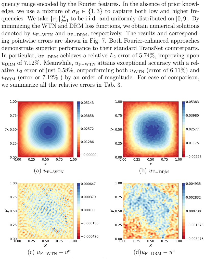
- Adding Fourier features (F-WTN) drops the multiscale Darcy-flow relative error from about 6.1e-2 to 5.8e-3, an order-of-magnitude improvement over standard WTN and the other comparators in the paper.
- Partition-of-unity localization with interface constraints reduces the sharp-gradient Poisson error to 1.35e-4 and, with mixed shape parameters, reduces the L-shape singular problem error to 3.06e-4.
- For nonlinear operators, the same least-squares kernel can be wrapped in Picard iteration, linearizing around the current approximation at each step and reusing the linear solve.
Reading between the lines
- Editorial extension: the paper does not supply an inf-sup condition or a priori error estimate, so the empirical accuracy may not persist for high-contrast coefficients or irregular domains beyond the tested cases.
- Editorial extension: the bilinear form printed in Sec. 5.2 writes the boundary term as -integral over dOmega of psi_i dphi_j/dn ds without the permeability kappa, which is inconsistent with integration by parts for -div(kappa grad u); if that formula is what was implemented, the reported experiments may solve a slightly modified operator.
- Editorial extension: the mixing of shape parameters in PoU-WTN suggests a cheap way to construct multiscale trial spaces without tuning a single gamma, and this idea could transfer to other random-feature PDE methods.
- Editorial extension: a natural testable extension is to apply F-WTN and PoU-WTN to time-dependent or nonlinear elliptic problems, or to choose RBF centers adaptively based on the weak residual, which the paper does not explore.
Editorial analysis
A structured set of objections, weighed in public.
Referee Report
Summary. This paper proposes a Petrov-Galerkin neural network method, Weak TransNet (WTN), for elliptic PDEs. The trial space is the neural feature space of a single-hidden-layer TransNet with frozen random weights, and the test space consists of radial basis functions; the coefficients are obtained by minimizing the weak residual in the least-squares sense with a soft boundary penalty. The paper also proposes two extensions: Fourier-WTN (F-WTN), which applies Fourier feature mapping to the TransNet inputs for multiscale problems, and PoU-WTN, which combines the method with a piecewise-constant partition of unity and interface penalties for problems with sharp gradients or singularities. The method is tested on 2D Darcy flow problems with discontinuous sources, multiscale permeability, channelized high-contrast permeability, a Poisson problem with a sharp gradient, and an L-shaped domain with a corner singularity, and is compared with strong-form and Ritz-energy TransNet baselines. The numerical experiments show that WTN and its extensions can be competitive and often more accurate than these baselines.
Significance. If the numerical results are supported by a consistent discretization, the paper offers an attractive workflow: for linear elliptic PDEs, the solution is obtained from a single linear least-squares solve, avoiding nonconvex optimization and the associated training difficulties. The reported gains are substantial, for example F-WTN reduces the multiscale Darcy error from 6.11% to 0.58%, and PoU-WTN with mixed shape parameters reduces the L-shape error from 4.30e-2 to 3.06e-4. The use of composite Simpson quadrature instead of Monte Carlo is a practical strength, and the paper is explicit about the empirical nature of the shape-parameter selection. However, the theoretical gaps and the incorrect boundary integral in Sec. 5.2 currently prevent the results from supporting the paper's central claim.
major comments (4)
- [§5.2, displayed formula for A_ij] The bilinear form A_ij = a(φ_j, ψ_i) = ∫_Ω κ∇φ_j·∇ψ_i dx − ∫_{∂Ω} ψ_i ∂φ_j/∂n ds omits the permeability κ from the boundary integral. For L[u] = −div(κ∇u), integration by parts gives ∫_Ω ψ L[u] dx = ∫_Ω κ∇u·∇ψ dx − ∫_{∂Ω} ψ κ ∂u/∂n ds. Since the RBF test functions do not vanish on ∂Ω and the boundary condition is only imposed as a soft penalty, the boundary term contributes to the discrete least-squares system. With κ ≠ 1 on ∂Ω, the corrected and displayed forms differ for any solution with a nonzero normal derivative, so the method as written solves a different boundary-value problem in general. The Sec. 5.2 experiment is insensitive to this error because the exact solution is independent of y and has zero normal derivative on all four boundary segments; the reported tables therefore do not validate the displayed formula. The bilinear form should be corrected and the experiments rerun for data with nonzero boundary flux.
- [§3, Eqs. (6)–(8)] The paper provides no stability or error analysis for the least-squares Petrov-Galerkin system. The method minimizes ∥Aα−f∥_2^2 with a boundary penalty, but no discrete inf-sup condition linking the RBF test space to U_TN is stated, no relation between N and M is derived, and no bound on the combined quadrature and boundary-penalty errors is given. The experiments only suggest that N slightly larger than M works well. The claim that the minimizer of (6) approximates the weak solution is therefore not supported; at minimum, a consistency estimate and a stability condition should be supplied, or the paper should be framed as purely empirical.
- [§4.2, Eqs. (11)–(14) and Alg. 2] The PoU-WTN method enforces the interface continuity and flux conditions only through soft penalties, with λ fixed to 1 in all experiments. No analysis is given for the consistency of this penalty formulation with the weak problem, and no sensitivity study with respect to λ is reported. Since the strong results in Secs. 5.4–5.6 depend on these interface constraints, the reader cannot assess whether the accuracy is robust or an artifact of the chosen penalty weight. A discretization error estimate or a systematic λ-study is needed.
- [§3.1 and §5.2–5.6] The stiffness and load entries are computed by composite Simpson quadrature on truncated RBF supports (N_l = 10), but no quadrature error analysis is provided. The support truncation itself introduces a modeling error because the Gaussian tails outside Ω_ψ are discarded, and this error is not quantified. A convergence study with respect to N_l and the Simpson mesh size would establish that the reported errors are not dominated by quadrature.
minor comments (10)
- [Abstract] The abstract cites 'Zhang et al., 2023' but reference [1] is dated 2024; please align the citation.
- [§3.1] There is a typo: 'homoegeneous' should be 'homogeneous'.
- [Algorithm 1] Lines 5 and 7 contain duplicated 'the the'; the wording should be cleaned up.
- [Figure 4 caption] The caption labels panels (a), (c), (d), (e), (f), (g) with no panel (b); the panel numbering should be corrected.
- [§5.2] The sentence 'The weight β for the boundary loss is set to as 1' should be 'set to 1'.
- [§5.3] In the discussion after Fig. 7, 'error or 7.12%' should be 'error of 7.12%'.
- [§5.6] The sentence 'the shape parameter for all neurons are to set to 1' should be 'the shape parameters for all neurons are set to 1'.
- [§4.2] The phrase 'partity of unity' should be 'partition of unity'.
- [§4.2] The symbol M denotes both the total number of localized basis functions and the number of trial basis functions in earlier sections; this overloaded notation should be clarified.
- [Appendix B] The formula for α* writes (L_DRM^T L_DRM)^{-1}; the text mentions adding a perturbation ϵI for numerical stability, but the displayed formula does not include it. Please update the equation.
Circularity Check
No significant circularity: the WTN coefficients are determined by a linear least-squares weak residual with fixed trial/test spaces, not by fitting the reported solutions.
full rationale
The central derivation is a direct Petrov-Galerkin least-squares formulation: the trial space is the frozen TransNet feature space, the test space is a set of RBFs, and the coefficients are obtained by minimizing the weak residual against the PDE data. The reported solutions are evaluated on separate test grids against exact or FEM reference solutions, so the accuracy claims are not forced by construction. The shape parameter gamma is selected on auxiliary Gaussian projection problems rather than on the target PDE, so its choice is a hyperparameter study, not a disguised fit. The paper relies on TransNet distributional results from [1] and [31]; these are prior published theorems and do not appear to involve the current authors. There is one minor self-citation, [20], used for the hard-constraint multiplier h=x(1-x)y(1-y) in the quadrature comparison, but that device is not load-bearing for the main error tables. A genuine consistency concern is present in Sec. 5.2, where the boundary term in Aij omits the permeability factor kappa (Aij = integral of kappa grad phi_j dot grad psi_i minus boundary integral of psi_i dphi_j/dn, while integration by parts for -div(kappa grad u) requires the boundary integrand psi_i kappa dphi_j/dn), and no inf-sup or consistency analysis is supplied. This is a correctness or validation gap, not a circular reduction: the method's predictions are not equivalent to its inputs by construction.
Assumptions & free parameters
free parameters (7)
- shape parameter gamma =
gamma=1 for smooth problems, gamma=5 for sharp gradients, mixture {1,5,10} near singularity
- RBF width sigma =
sigma=0.05, with 0.03 in Sec 3.1
- truncation factor N_l =
10
- boundary penalty weight beta =
1 for WTN and PoU-WTN; optimized for SF and DRM baselines
- interface penalty weight lambda =
1
- Fourier feature dimension P and frequency sigma_B =
P=64, sigma_B in {1,3}
- trial and test basis counts M and N =
M=100 to 2000, N=50 to 2000 depending on experiment
assumptions (5)
- domain assumption Existence and uniqueness of weak solutions for the elliptic boundary value problems considered.
- standard math Random hyperplane construction yields uniformly distributed neural basis functions (Theorem 1 of [1], Theorem 2 of [31]).
- ad hoc to paper The finite-dimensional least-squares Petrov-Galerkin system is solvable and stable.
- ad hoc to paper The piecewise-constant partition-of-unity basis with soft interface penalties is consistent with the weak solution.
- ad hoc to paper Composite Simpson quadrature on truncated RBF supports is accurate enough for the stiffness matrix.
Cite this review
Pith. "Pith review of Weak TransNet: A Petrov-Galerkin based neural network method for solving elliptic PDEs." pith.science (2026). https://pith.science/paper/4ITPVFLP
@misc{pith2026250614812,
  author       = {Pith},
  title        = {Pith review of: Weak TransNet: A Petrov-Galerkin based neural network method for solving elliptic PDEs},
  year         = {2026},
  howpublished = {\url{https://pith.science/paper/4ITPVFLP}},
  note         = {Machine review of arXiv:2506.14812}
}
read the original abstract
While deep learning has achieved remarkable success in solving partial differential equations (PDEs), it still faces significant challenges, particularly when the PDE solutions have low regularity or singularities. To address these issues, we propose the Weak TransNet (WTN) method, based on a Petrov-Galerkin formulation, for solving elliptic PDEs in this work, though its framework may extend to other classes of equations. Specifically, the neural feature space defined by TransNet (Zhang et al., 2023) is used as the trial space, while the test space is composed of radial basis functions. Since the solution is expressed as a linear combination of trial functions, the coefficients can be determined by minimizing the weak PDE residual via least squares. Thus, this approach could help mitigate the challenges of non-convexity and ill-conditioning that often arise in neural network training. Furthermore, the WTN method is extended to handle problems whose solutions exhibit multiscale features or possess sharp variations. Several numerical experiments are presented to demonstrate the robustness and efficiency of the proposed methods.
Figures


Figures from the paper (12 more)




Reference graph
Works this paper leans on
- [19]
- [1]
-
[2]
S. Whitaker, Flow in porous media I: A theoretical derivation of Darcy’s law, Transport in porous media 1 (1986) 3–25
work page 1986
-
[3]
Y. Efendiev, J. Galvis, T. Y. Hou, Generalized multiscale finite element methods (GMsFEM), Journal of computational physics 251 (2013) 116– 135
work page 2013
-
[4]
C. Yang, X. Yang, X. Xiao, Data-driven projection method in fluid simulation, Computer Animation and Virtual Worlds 27 (3-4) (2016) 415–424. 38
work page 2016
-
[5]
Y. Zhu, N. Zabaras, Bayesian deep convolutional encoder–decoder net- works for surrogate modeling and uncertainty quantification, Journal of Computational Physics 366 (2018) 415–447
work page 2018
-
[6]
Y. Zhu, N. Zabaras, P.-S. Koutsourelakis, P. Perdikaris, Physics- constrained deep learning for high-dimensional surrogate modeling and uncertainty quantification without labeled data, Journal of Computa- tional Physics 394 (2019) 56–81
work page 2019
-
[7]
Raissi, P
M. Raissi, P. Perdikaris, G. E. Karniadakis, Physics-informed neural networks: A deep learning framework for solving forward and inverse problems involving nonlinear partial differential equations, Journal of Computational physics 378 (2019) 686–707
2019
Show all 45 references
-
[8]
Y. Chen, B. Hosseini, H. Owhadi, A. M. Stuart, Solving and learn- ing nonlinear PDEs with Gaussian processes, Journal of Computational Physics 447 (2021) 110668
2021
-
[9]
S. Mo, Y. Zhu, N. Zabaras, X. Shi, J. Wu, Deep convolutional encoder- decoder networks for uncertainty quantification of dynamic multiphase flow in heterogeneous media, Water Resources Research 55 (1) (2019) 703–728
2019
-
[10]
S. Cai, Z. Mao, Z. Wang, M. Yin, G. E. Karniadakis, Physics-informed neural networks (PINNs) for fluid mechanics: A review, Acta Mechanica Sinica 37 (12) (2021) 1727–1738
2021
-
[11]
DeVore, B
R. DeVore, B. Hanin, G. Petrova, Neural network approximation, Acta Numerica 30 (2021) 327–444
2021
-
[12]
Rahaman, A
N. Rahaman, A. Baratin, D. Arpit, F. Draxler, M. Lin, F. Hamprecht, Y. Bengio, A. Courville, On the spectral bias of neural networks, in: International conference on machine learning, PMLR, 2019, pp. 5301– 5310
2019
-
[13]
Z.-Q. J. Xu, Y. Zhang, T. Luo, Y. Xiao, Z. Ma, Frequency principle: Fourier analysis sheds light on deep neural networks, arXiv preprint arXiv:1901.06523 (2019). 39
2019 arXiv
-
[14]
Sirignano, K
J. Sirignano, K. Spiliopoulos, DGM: A deep learning algorithm for solv- ing partial differential equations, Journal of computational physics 375 (2018) 1339–1364
2018
-
[15]
Yu, et al., The deep Ritz method: a deep learning-based numerical algorithm for solving variational problems, Communications in Mathe- matics and Statistics 6 (1) (2018) 1–12
B. Yu, et al., The deep Ritz method: a deep learning-based numerical algorithm for solving variational problems, Communications in Mathe- matics and Statistics 6 (1) (2018) 1–12
2018
-
[16]
Y. Zang, G. Bao, X. Ye, H. Zhou, Weak adversarial networks for high- dimensional partial differential equations, Journal of Computational Physics 411 (2020) 109409
2020
-
[17]
Kharazmi, Z
E. Kharazmi, Z. Zhang, G. E. Karniadakis, hp-VPINNs: Variational physics-informed neural networks with domain decomposition, Com- puter Methods in Applied Mechanics and Engineering 374 (2021) 113547
2021
-
[18]
Sheng, C
H. Sheng, C. Yang, PFNN: A penalty-free neural network method for solving a class of second-order boundary-value problems on complex geometries, Journal of Computational Physics 428 (2021) 110085
2021
-
[20]
P. Liu, Z. Xu, Z. Sheng, Subspace method based on neural networks for solving the partial differential equation in weak form, arXiv preprint arXiv:2405.08513 (2024)
2024 arXiv
-
[21]
Y. Liao, P. Ming, Deep Nitsche method: Deep Ritz method with essen- tial boundary conditions, arXiv preprint arXiv:1912.01309 (2019)
2019 arXiv
-
[22]
N. Wang, D. Zhang, H. Chang, H. Li, Deep learning of subsurface flow via theory-guided neural network, Journal of Hydrology 584 (2020) 124700
2020
-
[23]
R. Xu, D. Zhang, M. Rong, N. Wang, Weak form theory-guided neural network (TgNN-wf) for deep learning of subsurface single-and two-phase flow, Journal of Computational Physics 436 (2021) 110318. 40
2021
-
[24]
Z. Liu, W. Cai, Z.-Q. J. Xu, Multi-scale deep neural network (MscaleDNN) for solving Poisson-Boltzmann equation in complex do- mains, arXiv preprint arXiv:2007.11207 (2020)
2020 arXiv
-
[25]
B. Wang, W. Zhang, W. Cai, Multi-scale deep neural network (MscaleDNN) methods for oscillatory stokes flows in complex domains, arXiv preprint arXiv:2009.12729 (2020)
2020 arXiv
-
[26]
M.Raissi, P.Perdikaris, G.E.Karniadakis, Physicsinformeddeeplearn- ing (part I): Data-driven solutions of nonlinear partial differential equa- tions, arXiv preprint arXiv:1711.10561 (2017)
2017 arXiv
-
[27]
Markidis, The old and the new: Can physics-informed deep-learning replace traditional linear solvers?, Frontiers in big Data 4 (2021) 669097
S. Markidis, The old and the new: Can physics-informed deep-learning replace traditional linear solvers?, Frontiers in big Data 4 (2021) 669097
2021
-
[28]
S. Dong, Z. Li, Local extreme learning machines and domain decom- position for solving linear and nonlinear partial differential equations, Computer Methods in Applied Mechanics and Engineering 387 (2021) 114129
2021
-
[29]
J. Chen, X. Chi, Z. Yang, et al., Bridging traditional and ma- chine learning-based algorithms for solving PDEs: the random feature method, J Mach Learn 1 (2022) 268–98
2022
-
[30]
Y. Wang, S. Dong, An extreme learning machine-based method for com- putational PDEs in higher dimensions, Computer Methods in Applied Mechanics and Engineering 418 (2024) 116578
2024
-
[31]
T. Lu, L. Ju, L. Zhu, A multiple transferable neural network method with domain decomposition for elliptic interface problems, Journal of Computational Physics 530 (2025) 113902
2025
-
[32]
S. Ding, H. Zhao, Y. Zhang, X. Xu, R. Nie, Extreme learning ma- chine: algorithm, theory and applications, Artificial Intelligence Review 44 (2015) 103–115
2015
-
[33]
P. B. Bochev, M. D. Gunzburger, Least-squares finite element methods, Vol. 166, Springer Science & Business Media, 2009
2009
-
[34]
Kharazmi, Z
E. Kharazmi, Z. Zhang, G. E. Karniadakis, Variational physics-informed neural networks for solving partial differential equations, arXiv preprint arXiv:1912.00873 (2019). 41
2019 arXiv
-
[35]
Shang, F
Y. Shang, F. Wang, Randomized neural networks with Petrov–Galerkin methods for solving linear elasticity and Navier–Stokes equations, Jour- nal of Engineering Mechanics 150 (4) (2024) 04024010
2024
-
[36]
J. P. Roop, A randomized neural network based Petrov–Galerkin method for approximating the solution of fractional order boundary value problems, Results in Applied Mathematics 23 (2024) 100493
2024
-
[37]
Krishnapriyan, A
A. Krishnapriyan, A. Gholami, S. Zhe, R. Kirby, M. W. Mahoney, Char- acterizing possible failure modes in physics-informed neural networks, Advances in neural information processing systems 34 (2021) 26548– 26560
2021
-
[38]
M. D. Buhmann, Radial basis functions, Acta numerica 9 (2000) 1–38
2000
-
[39]
Tancik, P
M. Tancik, P. Srinivasan, B. Mildenhall, S. Fridovich-Keil, N. Raghavan, U. Singhal, R. Ramamoorthi, J. Barron, R. Ng, Fourier features let networks learn high frequency functions in low dimensional domains, Advances in neural information processing systems 33 (2020) 7537–7547
2020
-
[40]
S. Wang, H. Wang, P. Perdikaris, On the eigenvector bias of fourier fea- ture networks: From regression to solving multi-scale pdes with physics- informedneuralnetworks, ComputerMethodsinAppliedMechanicsand Engineering 384 (2021) 113938
2021
-
[41]
S. Li, Y. Xia, Y. Liu, Q. Liao, A deep domain decomposition method based on fourier features, Journal of Computational and Applied Math- ematics 423 (2023) 114963
2023
-
[42]
J. M. Melenk, I. Babuška, The partition of unity finite element method: basic theory and applications, Computer methods in applied mechanics and engineering 139 (1-4) (1996) 289–314
1996
-
[43]
Alnæs, J
M. Alnæs, J. Blechta, J. Hake, A. Johansson, B. Kehlet, A. Logg, C. Richardson, J. Ring, M. E. Rognes, G. N. Wells, The fenics project version 1.5, Archive of Numerical Software 3 (100) (2015)
2015
-
[44]
W. T. Leung, G. Lin, Z. Zhang, NH-PINN: Neural homogenization- based physics-informed neural network for multiscale problems, Journal of Computational Physics 470 (2022) 111539. 42
2022
-
[45]
L. Lu, R. Pestourie, W. Yao, Z. Wang, F. Verdugo, S. G. Johnson, Physics-informed neural networks with hard constraints for inverse de- sign, SIAMJournalon ScientificComputing43(6)(2021)B1105–B1132. 43
2021
Reviewed August 7, 2026 · model on record in the stance chip above.
Discussion (0). Sign in to comment.