REVIEW 5 major objections 5 minor 46 references
Photometric Redshift Predictions with a Neural Network for DESI Quasars
T0 review · 5 major / 5 minor · reviewed 2026-08-06 · deepseek-v4-flash
Pith's one-line read Adding GALEX ultraviolet photometry to DESI and WISE bands improves neural-network photometric redshifts for quasars, cutting scatter and catastrophic outliers.
desk verdict The GALEX improvement is real in direction, but the headline numbers compare different training samples, so the magnitude is unproven and there are internal numeric inconsistencies. read the letter →
The pith
A machine-rendered reading of the paper's core claim, the machinery that carries it, and where it could break.
The reading
What carries the argument
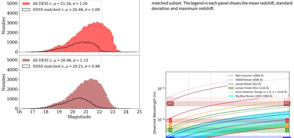
The machinery is a three-layer fully connected neural network with 200 neurons per hidden layer, ReLU activations, MSE loss, the Adam optimiser, and early stopping, trained on 80 per cent of the sample over 100 random train/test splits with K-fold cross-validation. The physical mechanism carrying the argument is the wide wavelength baseline from GALEX FUV (λ ≈ 1575 Å) through DESI g, r, z to WISE W1, W2 (λ ≈ 4.6 μm): as redshift increases, rest-frame UV features such as the Lyman break at 1216 Å and the Mg II line at 2800 Å move through these bands, so the added UV bands break colour–redshift degeneracies that a purely optical–infrared set leaves open. The paper deliberately uses raw fluxes and magnitudes rather than colour indices, arguing that this avoids introducing extra feature correlations while retaining the most fundamental observational data.
What would settle it
Train the same neural network on the DxS sample twice, once with g, r, z, W1, W2 only and once with FUV and NUV added, holding all sources and hyperparameters fixed; if the correlation and normalised median absolute deviation do not improve by roughly the amount implied by Table 9b (NMAD from about 0.32 to about 0.27), or if the improvement does not persist when the model is applied to faint, non-SDSS-matched DESI quasars, then the headline gain is largely a sample-selection effect rather than a true benefit of ultraviolet photometry.
Extended reading notes
Core claim
The central claim is that adding GALEX FUV and NUV photometry to DESI g, r, z and WISE W1, W2 fluxes substantially improves photometric redshift predictions for quasars: for a fully connected three-layer neural network, the correlation with spectroscopic redshift rises from r = 0.8099 on the DESI-only sample to r = 0.9187 on the DESI+GALEX sample, normalised median absolute deviation falls from 0.278 to 0.197, and the maximum and mean absolute errors both improve. The neural network also outperforms a tuned k-nearest-neighbours model on the same features. The authors attribute the gain to the wavelength lever arm from FUV (rest-frame 1575 Å) to W2, which lets the model span the Lyman break and other rest-frame UV features as they redshift through the observed bands. A secondary claim is that the bimodality seen in the optical-only predictions, driven by separation in the g–r versus z–W1 colour plane, is reduced when UV bands are included, and that when DESI and SDSS spectroscopic redshifts disagree, the photometric prediction agrees with DESI for about 73 per cent of the 107 outliers.
Load-bearing premise
The conclusion that GALEX ultraviolet bands cause the improvement assumes that the gain measured on the smaller, brighter SDSS-matched subset would also appear on the full DESI sample; the paper itself notes in Section 4.2 that GALEX-detected quasars are already among the brighter, better-constrained objects.
Editorial extensions
If this is right
- Photometric redshifts of quasars from a neural network are accurate enough that large surveys without full spectroscopic coverage can statistically use them for quasar samples.
- Deep ultraviolet photometry is more valuable than additional optical bands for quasar redshift estimation, since the network on DESI+GALEX outperforms the comparable model using SDSS ugriz alone.
- The bimodal structure in redshift predictions, tied to g–r versus z–W1 colours, means that explicitly modelling two quasar populations could further improve accuracy.
- When DESI and SDSS spectroscopic redshifts disagree, the nine-band photometric prediction sides with DESI for about 73 per cent of the 107 outliers, suggesting DESI's line associations are generally the more reliable ones.
Reading between the lines
- The comparison that carries the headline gain mixes two changes at once: the added ultraviolet bands and a switch from the full 87,318-source DESI sample to the smaller, brighter, better-constrained 24,616-source DxS subset; a clean test of the GALEX contribution would retrain the same architecture on the DxS sample with and without FUV/NUV, and the paper's own drop-column results on that fixed sa
- Permutation importance places FUV and NUV near the bottom even though add/remove comparisons show they matter, a known failure mode for correlated features; future redshift-model papers should report drop-column or Shapley-value importances alongside permutation scores.
- For radio-selected quasar samples expected from next-generation surveys, the same architecture could be retrained, but the selection-bias issue will be more severe because radio-selected samples have different redshift and luminosity distributions.
Editorial analysis
A structured set of objections, weighed in public.
Referee Report
Summary. This paper trains fully connected neural-network and k-nearest-neighbour regressors to predict photometric redshifts for DESI EDR quasars, using DESI g, r, z and WISE W1, W2 fluxes, optionally augmented with GALEX FUV and NUV fluxes obtained through a cross-match with SDSS DR16Q (the DxS subset of 24,616 sources). The authors report that adding GALEX photometry improves the neural network from r=0.8099 and NMAD=0.2781 on the full DESI sample to r=0.9187 and NMAD=0.1971 on DxS, and interpret this as evidence that ultraviolet coverage helps. They also examine redshift-dependent performance, a bimodality in the predictions, feature importances via permutation and drop-column methods, and use of the model to adjudicate between discrepant DESI and SDSS spectroscopic redshifts.
Significance. If the comparison were controlled, the result would be a useful practical demonstration that adding ultraviolet photometry to optical plus infrared quasar photometry improves photometric redshifts, with potential value for future wide surveys. The paper has genuine strengths: 100 randomized train/test runs, multiple standard metrics, held-out evaluation for the main comparisons, and feature-importance analysis with two complementary methods, including the more reliable drop-column approach. However, the headline quantitative claim is not supported as presented because the main GALEX comparison changes both the feature set and the training sample, and the appendix's same-sample check both shows a smaller effect and is internally inconsistent with the main table. The qualitative conclusion that ultraviolet photometry helps is plausible and consistent with the direction of Table 9, but the magnitude of the improvement needs to be re-established with a controlled and internally consistent comparison.
major comments (5)
- [§3.3; Tables 4 and 6 vs Table 9] The central claim that adding GALEX ultraviolet photometry improves the neural network from NMAD 0.278 to 0.197 rests on a comparison across different training samples: Table 4 uses the full 87,318-source DESI sample with (g,r,z,W1,W2), while Table 6 uses the 24,616-source DxS subset with (g,r,z,W1,W2,FUV,NUV). Because Section 4.2 acknowledges that GALEX-detected quasars are brighter and better constrained, the improvement conflates added bands with an easier sample. The same-sample check in Table 9b shows a much smaller effect on DxS, NMAD 0.3171 without ultraviolet photometry versus 0.2699 with it, about 15% rather than 29%, so the headline magnitude is not established. Please re-run the DESI-only model on the same DxS subset used for the GALEX model and report both comparisons.
- [Table 9b vs Table 6] Table 9b gives a neural-network NMAD of 0.2699 for the feature set (g,r,z,W1,W2,FUV,NUV) on DxS, whereas Table 6 reports 0.1971 for what appears to be the same feature set and dataset; these two values cannot both describe the same configuration. Table 9a's kNN baseline of 0.2584 matches Table 6's kNN GALEX value, ruling out a simple across-the-board formatting difference. Please clarify whether Table 9b uses a different sample, a single run, a different network, or a different training pipeline, and reconcile the discrepancy.
- [Table 7; Eq. (1)] The percentage changes in Table 7 contradict Eq. (1), which defines the improvement relative to the NN DESI baseline. For example, the NN DESI/GALEX NMAD is reported as -41.1%, but Eq. (1) gives (0.1971 - 0.2781)/0.2781 = -29.1%; the correlation coefficient is reported as 11.84% instead of 13.4%. The Section 5 text, which states a 13% increase in correlation and a 29% reduction in NMAD, matches Eq. (1), but Table 7 and the surrounding discussion, which says all metrics improve by about 40%, do not. Correct the table and the related sentences.
- [§4.4; Figures 13-14; Conclusion] The outlier-adjudication claim is partly circular. The model whose predictions are used in Figures 13 and 14 was trained with zDESI as the target on the DxS sample after removing the 107 outliers, as described in Section 4.4, so a tendency for zphot to sit closer to zDESI than to zSDSS is expected even if the two spectroscopic measurements are equally accurate. To support the conclusion that DESI redshifts are more reliable in the discrepant cases, train a comparison model on zSDSS or validate the outlier assignments against an independent redshift source.
- [§2.6-2.7] Model selection appears to use the test set directly: Section 2.6 states that the neural-network architecture was chosen based on the lowest RMS error on the test set, and Section 2.7 states that the kNN hyperparameters were optimized to minimize RMS error on the test set. If the reported metrics are computed on the same test set used for selection, the absolute performance values are likely optimistic. Please use a separate validation split for hyperparameter selection and report test-set metrics from the final selected configuration.
minor comments (5)
- [§2.5] The definition of explained variance is malformed as printed: the expression for sigma-squared of the residuals lacks a division by N and appears to use zspec in the denominator; please restate it consistently with the residual definition Delta-z = zspec - zphot.
- [§2.6 / Figure 5] The text says architectures with 1 to 6 hidden layers and 50 to 300 neurons per layer were explored, but the final architecture is only given in Figure 5; please state the number of layers, neurons per layer, activation function, optimizer, and early-stopping details in the text.
- [§3.1] The symbol sigma-prime-z is introduced without definition in Section 3.1, where the text reports low scatter of sigma-prime-z = 0.387; define it or replace it with a metric defined in Section 2.5.
- [References] There is a typo in the introduction, W olf, in the reference to Wolf et al. 2018, and the reference list contains entries for Duncan 2021 and Duncan 2022 with only one clearly cited in the text; please clean up the bibliography.
- [Abstract / §5] The abstract and conclusions present r=0.9187 and NMAD=0.197 without stating that these values are for the DxS subset rather than the full DESI sample; please state the sample explicitly to avoid over-generalization.
Circularity Check
Main photo-z evaluation uses held-out test data and is not circular; one secondary outlier-reliability claim is biased by training on the very redshift catalog it endorses, and self-citations are not load-bearing.
-
fitted input called prediction
[Section 4.4, 'Predicting redshift for outliers in DESI/SDSS crossmatched sources' (Figures 13 and 14)]
"To address the mismatches in the DESI and SDSS redshifts, we remove the 107 problematic sources and retrain our model on the remaining 24509 sources, using the DESI spectroscopic redshift (zDESI) as the target. Figure 13 shows a diagnostic scatterplot comparing the photometric redshift accuracy and photometric consistency for the outlier QSOs, showing that for 78 out of 107 (∼ 73%) outliers, our predictions most closely match the DESI spectroscopic redshift."
The model's regression target is zDESI, so the photometric redshifts are fitted to reproduce DESI spectroscopic redshifts on the training sample. Using those same zphot values to adjudicate between zDESI and zSDSS for the 107 outliers therefore has a built-in bias: zphot will tend to lie closer to the catalog on which it was trained, even if the photometry carries little independent redshift information. The claim that 'our predictions most closely match the DESI spectroscopic redshift' is thus partly enforced by the training target, not an independent test of which catalog is more reliable.
full rationale
The central photo-z results are not circular: the NN is trained on 80% of a given sample and evaluated on a held-out 20%, with metrics averaged over 100 shuffled runs (Section 2.5), which is a standard out-of-sample evaluation. The self-citations to Curran et al. (2021, 2022) and Curran (2022) support method choices such as raw fluxes and the network architecture, and they are not load-bearing for the UV-improvement claim. I do not count the GALEX comparison as circular: although the abstract's comparison of Table 4 (full DESI, 87318 sources) with Table 6 (DxS subset, 24616 sources, with GALEX) is confounded by sample selection, and Section 4.2 itself notes that GALEX-detected quasars are 'already among the brighter, better-constrained subset,' this is an experimental-design flaw rather than a reduction of a result to its inputs. Likewise, the inconsistency between Table 6 (NN+DxS+GALEX NMAD = 0.1971) and Table 9b's baseline for the same feature set (NMAD = 0.2699), and the Table 7 percentage changes that contradict Eq. (1), are correctness issues to be fixed by the authors, not circularity. The one mild circular step is the Section 4.4 outlier analysis, where the model is trained with zDESI as the target and then used to argue that zphot favors DESI over SDSS; that claim is biased by construction and is a secondary, partial circularity. Hence the overall score is 2: one minor non-load-bearing self-citation pattern and one secondary claim that is partly fitted-input-called-prediction, while the main photometric-redshift derivation remains self-contained.
Assumptions & free parameters
free parameters (3)
- NN architecture (layers, neurons) =
3 hidden layers, 200 neurons each
- kNN k, distance metric, weighting =
k=18, Manhattan, distance weighting
- Redshift outlier threshold =
0.14
assumptions (6)
- domain assumption Photometric redshifts are a function of broadband fluxes; ML can learn this mapping from spectroscopic training data.
- domain assumption The DxS crossmatch with a 1 arcsec radius correctly associates DESI and SDSS sources.
- domain assumption Standard astronomical data processing (extinction correction, flux standardization) preserves the information needed for redshift inference.
- domain assumption The held-out test set is representative of the full DESI quasar population.
- domain assumption DESI spectroscopic redshifts are the ground truth for training.
- standard math Neural network training with MSE loss and early stopping converges to a stable solution.
Cite this review
Pith. "Pith review of Photometric Redshift Predictions with a Neural Network for DESI Quasars." pith.science (2026). https://pith.science/paper/7M6KI3QI
@misc{pith2026250703260,
  author       = {Pith},
  title        = {Pith review of: Photometric Redshift Predictions with a Neural Network for DESI Quasars},
  year         = {2026},
  howpublished = {\url{https://pith.science/paper/7M6KI3QI}},
  note         = {Machine review of arXiv:2507.03260}
}
abstract
Accurate redshift measurements are essential for studying the evolution of quasi-stellar objects (QSOs) and their role in cosmic structure formation. While spectroscopic redshifts provide high precision, they are impractical for the vast number of sources detected in large-scale surveys. Photometric redshifts, derived from broadband fluxes, offer an efficient alternative, particularly when combined with machine learning techniques. In this work, we develop and evaluate a neural network model for predicting the redshifts of QSOs in the Dark Energy Spectroscopic Instrument (DESI) Early Data Release spectroscopic catalogue, using photometry from DESI, the Widefield Infrared Survey Explorer (WISE) and the Galactic Evolution Explorer (GALEX). We compare the performance of the neural network model against a k-Nearest Neighbours approach, these being the most accurate and least resource-intensive of the methods trialled herein, optimising model parameters and assessing accuracy with standard statistical metrics. Our results show that incorporating ultraviolet photometry from GALEX improves photometric redshift estimates, reducing scatter and catastrophic outliers compared to models trained only on near infrared and optical bands. The neural network achieves a correlation coefficient with spectroscopic redshift of $0.9187$ with normalised median absolute deviation of $0.197$, representing a significant improvement over other methods. Our work combines DESI, WISE and GALEX measurements, providing robust predictions which address the difficulties in predicting photometric redshift of QSOs over a large redshift range.
Figures


Figures from the paper (15 more)


Reference graph
Works this paper leans on
-
[1]
Abadi, M., Agarwal, A., Barham, P., et al. 2016, TensorFlow: Large-Scale Machine Learning on Heterogeneous Distributed Systems, arXiv:1603.04467
arXiv 2016
-
[2]
2022, The Astronomical Journal, 164, 207
Abareshi, B., Aguilar, J., Ahlen, S., et al. 2022, The Astronomical Journal, 164, 207
work page 2022
-
[3]
G., Aguilar, J., Ahlen, S., et al
Adame, A. G., Aguilar, J., Ahlen, S., et al. 2023, arXiv e-prints, doi:10.48550/ARXIV.2306.06308
-
[4]
Alexander, D. M., Davis, T. M., Chaussidon, E., et al. 2023, The Astronomical Journal, 165, 124
work page 2023
- [5]
-
[6]
Ball, N. M., Brunner, R. J., Myers, A. D., et al. 2008, The Astrophysical Journal, 683, 12 —. 2007, The Astrophysical Journal, 663, 774
work page 2008
-
[7]
2023, Bird’s Convention for Diagramatic Neural Networks
Bird, G. 2023, Bird’s Convention for Diagramatic Neural Networks
work page 2023
-
[8]
Bovy, J., Myers, A. D., Hennawi, J. F., et al. 2012, The Astrophysical Journal, 749, 41
work page 2012
Show all 46 references
-
[9]
B., van Dokkum, P
Brammer, G. B., van Dokkum, P. G., & Coppi, P. 2008, The Astrophysical Journal, 686, 1503
2008
-
[10]
2021, Frontiers in Astronomy and Space Sciences, 8, arXiv:2104.06774
Brescia, M., Cavuoti, S., Razim, O., et al. 2021, Frontiers in Astronomy and Space Sciences, 8, arXiv:2104.06774
2021 arXiv
- [11]
-
[12]
2004, arXiv e-prints, 1
Carilli, C., & Rawlings, S. 2004, arXiv e-prints, 1
2004
-
[13]
2007, Astronomical Data Analysis Software and Systems, arXiv:0711.2477v1
Carliles, S., Heinis, S., & Priebe, C. 2007, Astronomical Data Analysis Software and Systems, arXiv:0711.2477v1
2007 arXiv
-
[14]
2023, The Astrophysical Journal, 944, 107
Chaussidon, E., Yèche, C., Palanque-Delabrouille, N., et al. 2023, The Astrophysical Journal, 944, 107
2023
-
[15]
J., & Szalay, A
Connolly, A. J., & Szalay, A. S. 1999, The Astronomical Journal, 117, 2052
1999
-
[16]
Curran, S. J. 2020, Monthly Notices of the Royal Astronomical Society: Letters, 493, L70 —. 2022, Monthly Notices of the Royal Astronomical Society, 12, 1
2020
-
[17]
J., Moss, J
Curran, S. J., Moss, J. P., & Perrott, Y. C. 2021, Monthly Notices of the Royal Astronomical Society, 503, 2639 —. 2022, Monthly Notices of the Royal Astronomical Society, 514, 1
2021
-
[18]
2021, TensorFlow, Zenodo, doi:10.5281/zenodo.4758419
Developers, T. 2021, TensorFlow, Zenodo, doi:10.5281/zenodo.4758419
2021 doi
-
[19]
J., Lang, D., et al
Dey, A., Schlegel, D. J., Lang, D., et al. 2019, The Astronomical Journal, 157, 168 D’Isanto, A., & Polsterer, K. L. 2018, Astronomy and Astrophysics, 609, A111
2019
-
[20]
2010, Astronomische Nachrichten, 331, 535
Dravins, D. 2010, Astronomische Nachrichten, 331, 535
2010
-
[21]
Duncan, K. J. 2021, 20, 1 —. 2022, Monthly Notices of the Royal Astronomical Society, 512, 3662 Gil de Paz, A., Boissier, S., Madore, B. F., et al. 2007, The Astrophysical Journal Supplement Series, 173, 185
2021
-
[22]
2016, Research in Astronomy and Astrophysics, 16, 005
Han, B., Ding, H.-P., Zhang, Y.-X., & Zhao, Y.-H. 2016, Research in Astronomy and Astrophysics, 16, 005
2016
-
[23]
2022, 10, 1
Hong, S., Zou, Z., Luo, A.-l., et al. 2022, 10, 1
2022
-
[24]
2015, Monthly Notices of the Royal Astronomical Society, 449, 1275
Hoyle, B., Michael Rau, M., Zitlau, R., Seitz, S., & Weller, J. 2015, Monthly Notices of the Royal Astronomical Society, 449, 1275
2015
-
[25]
P., & Ba, J
Kingma, D. P., & Ba, J. 2017, Adam: A Method for Stochastic Optimization, arXiv:1412.6980 Kügler, S. D., Gianniotis, N., & Polsterer, K. L. 2016, in 2016 IEEE Symposium Series on Computational Intelligence, SSCI 2016, Athens, Greece, December 6-9, 2016 (IEEE), 1–8
2017 arXiv
-
[26]
2022, 525, 513
Li, C., Zhang, Y., Cui, C., et al. 2022, 525, 513
2022
-
[27]
2023, Publications of the Astronomical Society of Australia, 40, 1
Luken, K., Norris, R., Wang, X., et al. 2023, Publications of the Astronomical Society of Australia, 40, 1
2023
-
[28]
J., Norris, R
Luken, K. J., Norris, R. P., Park, L. A. F., Wang, X. R., & Filipovic, M. D. 2022, Estimating Galaxy Redshift in Radio-Selected Datasets Using Machine Learning, arXiv:2202.13504
2022 arXiv
-
[29]
W., Higley, A
Lyke, B. W., Higley, A. N., McLane, J. N., et al. 2020, Astrophysical Journal Supplement Series, 250, 8
2020
-
[30]
C., Fanson, J., Schiminovich, D., et al
Martin, D. C., Fanson, J., Schiminovich, D., et al. 2005, The Astrophysical Journal, 619, L1
2005
-
[31]
R., Soares, G., et al
Nakazono, L., Valença, R. R., Soares, G., et al. 2024, Monthly Notices of the Royal Astronomical Society, stae971
2024
-
[32]
D., Jimenez, R., Verde, L., et al
Niemack, M. D., Jimenez, R., Verde, L., et al. 2009, The Astrophysical Journal, 690, 89
2009
-
[33]
P., Hopkins, A
Norris, R. P., Hopkins, A. M., Afonso, J., et al. 2011, Publications of the Astronomical Society of Australia, 28, 215
2011
-
[34]
2019, Astronomy and Astrophysics, 621, 1
Pasquet, J., Bertin, E., Treyer, M., Arnouts, S., & Fouchez, D. 2019, Astronomy and Astrophysics, 621, 1
2019
-
[35]
2018, Astronomy and Astrophysics, 611, 1
Pasquet-Itam, J., & Pasquet, J. 2018, Astronomy and Astrophysics, 611, 1
2018
-
[36]
2017, Publications of the Astronomical Society of the Pacific, 129, doi:10.1088/1538-3873/aa7843
Popowicz, A., & Kurek, A. 2017, Publications of the Astronomical Society of the Pacific, 129, doi:10.1088/1538-3873/aa7843
2017 doi
-
[37]
2024, Astronomy & Astrophysics, 690, A365
Saxena, A., Salvato, M., Roster, W., et al. 2024, Astronomy & Astrophysics, 690, A365
2024
-
[38]
Schilizzi, R. T. 2004, https://doi.org/10.1117/12.551206, 5489, 62
2004 doi
-
[39]
F., & Finkbeiner, D
Schlafly, E. F., & Finkbeiner, D. P. 2011, The Astrophysical Journal, 737, 103
2011
-
[40]
2021, 237, 235.03 W olf, C., Onken, C
Schlegel, D., Dey, A., Herrera, D., et al. 2021, 237, 235.03 W olf, C., Onken, C. A., Luvaul, L. C., et al. 2018, Publications of the Astronomical Society of Australia, 35, doi:10.1017/pasa.2018.5
2021 doi
-
[41]
L., Eisenhardt, P
Wright, E. L., Eisenhardt, P. R. M., Mainzer, A. K., et al. 2010, The Astronomical Journal, 140, 1868
2010
-
[42]
B., Liu, X
Yuan, H. B., Liu, X. W., & Xiang, M. S. 2013, Monthly Notices of the Royal Astronomical Society, 430, 2188
2013
-
[43]
2010, Monthly Notices of the Royal Astronomical Society, 408, 1283
Zhang, F., Han, Z., Li, L., Shan, H., & Zhang, Y. 2010, Monthly Notices of the Royal Astronomical Society, 408, 1283
2010
-
[44]
2013, The Astronomical Journal, 146, 22
Zhang, Y., Ma, H., Peng, N., Zhao, Y., & Wu, X.-b. 2013, The Astronomical Journal, 146, 22
2013
-
[45]
2019, Research in Astronomy and Astrophysics, 19, 175
Zhang, Y.-X., Zhang, J.-Y., Jin, X., & Zhao, Y.-H. 2019, Research in Astronomy and Astrophysics, 19, 175
2019
-
[46]
A., Mao, Y.-Y., et al
Zhou, R., Newman, J. A., Mao, Y.-Y., et al. 2021, Monthly Notices of the Royal Astronomical Society, 501, 3309
2021
Reviewed August 6, 2026 · model on record in the stance chip above.
Discussion (0). Sign in to comment.