REVIEW 3 major objections 6 minor 2 references
Spline Deformation Field
T0 review · 3 major / 6 minor · reviewed 2026-08-06 · deepseek-v4-flash
Pith's one-line read Representing dense point trajectories as cubic splines, with knot positions and tangents predicted by a coordinate network, beats implicit deep-feature interpolation on sparse temporal signals and improves spatial coherence in dynamic…
desk verdict Solid spline-based deformation representation with real interpolation gains, but the Moran's I metric as printed is not Moran's I and the coherence claims need a rework. read the letter →
The pith
A machine-rendered reading of the paper's core claim, the machinery that carries it, and where it could break.
The reading
What carries the argument
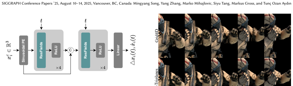
The load-bearing mechanism is the spline deformation field: a cubic Hermite spline between a start and end knot, where each knot carries a position and a tangent predicted by a coordinate network. The network uses time-variant spatial encoding: at timestep t, spatial features are decoded through base weights plus a low-rank residual sum over temporal codes, decoupling spatial and temporal information. Because the spline is polynomial in normalized time, velocity and acceleration are obtained by differentiating the interpolation function; these analytic derivatives feed a neighbor-consistent velocity loss and an acceleration magnitude loss. The knot count is tied to the training timestep count by K·N=T with K=2 for cubic Hermite, so N=T/2, which the paper argues makes the fit well-determined. This machinery turns trajectory modeling into an interpolation problem with explicit, physically meaningful derivatives rather than implicit network smoothness.
What would settle it
Train the same spline pipeline on DeformingThings4D with every 4th frame while sweeping N above and below T/2 (say N=T/4 and N=T); if some off-rule N matches or beats N=T/2 in EPE and Moran's I, or if the optimal N shifts with motion complexity, the degrees-of-freedom rule is empirically falsified.
Extended reading notes
Core claim
The paper's central object is a cubic Hermite spline applied to each point's trajectory over time: at knots t_start and t_end the network predicts both position offsets and tangents; query times are interpolated by a third-order polynomial. Choosing N=T/2 knots for T training timesteps is proposed as a degrees-of-freedom balance that avoids under- and over-fitting; the closed-form derivative of the spline then supplies velocity, used in a neighbor-consistency loss L_v, and acceleration, used as a jitter suppression loss L_acc. A low-rank time-variant spatial encoding (TVSE) replaces coupled 4D inputs, letting the same encoding run with sinusoidal positional encodings, dense grids, or residual field weights. The resulting spline field is evaluated on scene-flow interpolation and dynamic scene reconstruction with Gaussian splatting, where it outperforms deep-feature interpolation on sparse temporal inputs and raises a Moran's I spatial-coherence measure across NeRF-DS, Hyper-NeRF, and Neu3D.
Load-bearing premise
The method assumes that tying the knot count to N=T/2 makes the spline fit well-determined without heuristic tuning, yet for NeRF-DS the paper sets N=30 by hand; if the right N is dataset-dependent, the claimed advantage of explicit interpolation is partly a capacity choice.
Editorial extensions
If this is right
- On long-sequence scene-flow interpolation with every 4th or 6th frame as input, the spline field reports EPE 40.74/68.28, beating ResFields with AIAP at 45.72/73.00 and DOMA at 138.80/146.51.
- The explicit regularity terms extend to both MLP and grid backbones, so SF-PE-ResFields, SF-Triplanes, and SF-Triaxes all raise Moran's I on NeRF-DS, Hyper-NeRF, and Neu3D without linear blend skinning or as-rigid-as-possible constraints.
- Analytic velocity enables motion advection and trajectory editing with only keyframe edits, and coherent canonical-space deformations allow style transfer across the full sequence.
- The knot-counting rule N=T/2 is presented as eliminating heuristic knot selection and as a diagnostic tool: reducing N in large-motion data produces large misalignment that penalizes reconstruction accuracy.
Reading between the lines
- If the N=T/2 rule is genuine capacity accounting, knot count should generalize across sequences of different lengths; the paper's manual N=30 for NeRF-DS suggests the rule may instead be a tuned prior, and a knot sweep across datasets would clarify the distinction.
- Because TVSE is architecture-agnostic, the spline representation could be combined with hash grids or future encodings; the supplementary material already suggests time-variant spatial hash encoding as promising.
- Analytic velocity opens a natural interface to physics-based losses or simulation, a direction the paper only gestures at through advection experiments.
- Moran's I, as defined here, measures spatial autocorrelation of discrete motion vectors; treating it as a standard coherence metric for dynamic scene reconstruction would require checking its agreement with perceptual quality on more diverse scenes.
Editorial analysis
A structured set of objections, weighed in public.
Referee Report
Summary. The paper proposes a spline-based trajectory representation for dynamic point and scene reconstruction. Trajectories are modeled as cubic Hermite splines whose knot positions and tangents are predicted by a coordinate network; temporal conditioning is implemented through a low-rank time-variant spatial encoding (TVSE) applied to MLP, triplane, and triaxis backbones. Analytical derivatives of the spline yield velocity and acceleration regularizers. Experiments on DeformingThings4D scene-flow interpolation, NeRF-DS, Hyper-NeRF, Neu3D, and D-NeRF report improvements in endpoint error and a Moran's I-based spatial-coherence metric. The paper claims that explicit spline interpolation outperforms deep feature interpolation under sparse temporal sampling and improves spatial coherence without LBS or ARAP constraints.
Significance. If the results hold, the paper offers a simple, encoding-agnostic way to inject explicit temporal continuity into implicit deformation fields, with a clean degrees-of-freedom interpretation and cheap analytical regularizers. The reported EPE gains on DeformingThings4D (40.74/68.28 versus 45.72/73.00 for ResFields with AIAP, Table 1) are substantial and are independent of the coherence metric. The manuscript also provides detailed architecture descriptions and ablations. However, the paper's spatial-coherence evidence is compromised by the non-standard Moran's I formula in Eq. 12; until that is corrected, only the EPE-based interpolation claim is quantitatively supported.
major comments (3)
- [A.1, Eq. (12)] The quantity called Moran's I in Eq. (12) is not Moran's I as defined in the cited reference (Moran 1950). The standard statistic is I = (N/W) * sum_i sum_j w_ij (z_i - zbar)(z_j - zbar) / sum_i (z_i - zbar)^2. Equation (12) instead computes K/(sum_i sum_j w_ij) * (sum_i sum_j w_ij v_i dot v_j)/(sum_i v_i), using raw 3D offsets, no mean centering, and a denominator that is neither squared nor scalar. For vector-valued offsets this is dimensionally inconsistent, and an uncentered dot-product index is dominated by any common translation, so it can report high autocorrelation even for spatially random velocities superimposed on a global offset. Because Tables 1-4 and Figures 5-7 use this index to support the spatial-coherence half of the central claim, the printed formula makes those numbers uninterpretable. Please replace Eq. (12) with a correctly centered statistic (or a clearly specified and dimensionally consistent vector generalization), recompute all Moran's I values, and state explicitly whether the implementation matches the corrected formula.
- [Sec. 3.2.1 vs. Eq. (1) and App. D] The paper asserts that Eq. (1) with K=2, i.e., N=T/2, guarantees a well-determined fit and removes heuristic knot selection. This is contradicted by Sec. 3.2.1, where N=30 is set manually for NeRF-DS ('To account for the motion characteristics in this dataset, we set N = 30 and rank = 10'), and by App. D, which admits that 'the dense number of knots increases the risk of jittering in certain corner cases.' If N is a per-dataset hyperparameter, the advantage of the explicit representation is partly a capacity choice rather than a principled consequence of degree-of-freedom counting. Please reconcile the two statements, justify the manual N=30 choice in terms of the effective number of training timesteps, and provide a sensitivity study over N.
- [Sec. 2.3, Eqs. (6) and (8)] Equations (6) and (8) are derivatives with respect to the normalized time \bar{t}; the physical velocity and acceleration are (1/tau) v(\bar{t}) and (1/tau^2) a(\bar{t}), where tau = 1/(N-1) is the knot interval. Omitting these factors means the regularization losses L_v and L_acc have strengths that implicitly depend on N, and the claim that v has 'physical meaning' is imprecise. If the normalization is intentional, state it explicitly; if physical units are intended, include the interval factors in the loss definitions so that comparisons across different N and across datasets are not confounded by the missing 1/tau factors.
minor comments (6)
- [Table 1 caption] The caption contains a typo: 'DeformaingTings4D' should be 'DeformingThings4D', and the notation 'M. ’sI' is awkwardly formatted throughout the tables.
- [A.1, Eq. (12)] The index notation in Eq. (12) is unclear: the sums run over K neighbor indices, but the quantity is written as I_t(x_i), and the relationship between the outer point i and the neighbor set should be clarified.
- [Table 9, T-Rex row] The T-Rex row contains '34.22 FALSE 0.73' in the PSNR/SSIM/Moran's I columns, which appears to be a formatting error; these columns should contain numerical values or a clear explanation for missing entries.
- [Fig. 7 caption] The caption says 'preserve the handle with reflection batter than the baselines'; 'batter' should be 'better'.
- [Sec. 1 and Sec. 3.1] The text contains typos, including 'ResFileds' (should be 'ResFields') and 'concept on' (should be something like 'build on'); please proofread for these and similar errors.
- [A.3] The hyperparameter table (Table 6) lists alpha and beta per dataset, but the text also mentions learning-rate multipliers for grids and MLPs; adding these to the table or to the text would improve reproducibility.
Circularity Check
No significant circularity: interpolation EPE is evaluated on held-out timesteps, and the Moran's I metric concern is a correctness issue rather than a circular reduction.
full rationale
The paper's central quantitative claim is temporal interpolation (EPE) on DeformingThings4D, evaluated at timesteps withheld from training (75%/83.3% held out). The spline knots and tangents are predicted by a Coord.-NN and optimized by L1 reconstruction loss; the held-out positions are genuine interpolations between fitted knots, not re-statements of the training values. Velocity and acceleration losses (Eqs. 7, 9) are regularizers, not supervised predictions, and no fitted parameter is later renamed as a prediction. The low-rank TVSE (Eq. 5) is a modeling choice inspired by ResFields, not derived from the target outputs, and no uniqueness theorem is imported from the authors' prior work. Self-citations to ResFields, DOMA, and DPF are abundant, but they serve as baselines and architectural building blocks whose content is independently published and externally comparable, so they are not load-bearing circularity. One non-circular caveat: the Moran's I implementation in Appendix A.1, Eq. 12 is not the standard Moran's I (it omits mean-centering, uses raw vector offsets, and has a dimensionally inconsistent denominator), which undermines the spatial-coherence evidence; this is a metric-validity/correctness concern, not a circular derivation, so it does not increase the circularity score.
Assumptions & free parameters
free parameters (4)
- Number of knots N =
T/2 for scene flow; 30 for NeRF-DS; determined per dataset otherwise
- Rank of temporal codes =
60 for scene flow, 10 for NeRF-DS, 16 for Hyper-NeRF
- Loss weights alpha and beta =
alpha: 1.0, 0.01, 0.05, 0.0001; beta: 0.01, 0.1, 0.05, 0.05 across datasets (Table 6)
- Lambda for SSIM loss =
0.2
assumptions (6)
- standard math Cubic Hermite spline basis functions are used for interpolation (Eq. 2)
- domain assumption Uniform knot placement in time; knot positions are not optimized
- domain assumption Temporal encoding can be represented as a base plus a low-rank residual combination (Eq. 5)
- domain assumption Neighboring points in canonical space should have similar velocities (Eq. 7)
- ad hoc to paper Equation 1 (K*N=T) guarantees a well-determined spline fit
- ad hoc to paper Moran's I as computed in Eq. 12 measures spatial coherence
Cite this review
Pith. "Pith review of Spline Deformation Field." pith.science (2026). https://pith.science/paper/ONBILCOV
@misc{pith2026250707521,
  author       = {Pith},
  title        = {Pith review of: Spline Deformation Field},
  year         = {2026},
  howpublished = {\url{https://pith.science/paper/ONBILCOV}},
  note         = {Machine review of arXiv:2507.07521}
}
read the original abstract
Trajectory modeling of dense points usually employs implicit deformation fields, represented as neural networks that map coordinates to relate canonical spatial positions to temporal offsets. However, the inductive biases inherent in neural networks can hinder spatial coherence in ill-posed scenarios. Current methods focus either on enhancing encoding strategies for deformation fields, often resulting in opaque and less intuitive models, or adopt explicit techniques like linear blend skinning, which rely on heuristic-based node initialization. Additionally, the potential of implicit representations for interpolating sparse temporal signals remains under-explored. To address these challenges, we propose a spline-based trajectory representation, where the number of knots explicitly determines the degrees of freedom. This approach enables efficient analytical derivation of velocities, preserving spatial coherence and accelerations, while mitigating temporal fluctuations. To model knot characteristics in both spatial and temporal domains, we introduce a novel low-rank time-variant spatial encoding, replacing conventional coupled spatiotemporal techniques. Our method demonstrates superior performance in temporal interpolation for fitting continuous fields with sparse inputs. Furthermore, it achieves competitive dynamic scene reconstruction quality compared to state-of-the-art methods while enhancing motion coherence without relying on linear blend skinning or as-rigid-as-possible constraints.
Figures


Figures from the paper (15 more)




Reference graph
Works this paper leans on
-
[2022]
InProceedings of the IEEE/CVF Conference on Computer Vision and Pattern Recognition
Neural 3d video synthesis from multi-view video. InProceedings of the IEEE/CVF Conference on Computer Vision and Pattern Recognition . 5521–5531. Yang Li, Hikari Takehara, Takafumi Taketomi, Bo Zheng, and Matthias Nießner. 2021. 4dcomplete: Non-rigid motion estimation beyond the observable surface. In Pro- ceedings of the IEEE/CVF International Conference...
arXiv 2023
-
[2023]
arXiv preprint arXiv:2312.14937 (2023)
SC-GS: Sparse-Controlled Gaussian Splatting for Editable Dynamic Scenes. arXiv preprint arXiv:2312.14937 (2023). Matthias Innmann, Kihwan Kim, Jinwei Gu, Matthias Nießner, Charles Loop, Marc Stamminger, and Jan Kautz. 2020. Nrmvs: Non-rigid multi-view stereo. InProceedings of the IEEE/CVF Winter Conference on Applications of Computer Vision . 2754–2763. B...
arXiv 2023
Reviewed August 6, 2026 · model on record in the stance chip above.
Discussion (0). Continue with ORCID to comment.