REVIEW 4 major objections 8 minor 1 cited by
Adaptive feature capture method for solving partial differential equations with near singular solutions
T0 review · 4 major / 8 minor · reviewed 2026-08-06 · deepseek-v4-flash
Pith's one-line read After four gradient-guided resampling iterations, near-singular PDE solutions reach relative errors around $10^{-10}$.
desk verdict AFCM is a genuinely useful adaptive extension of RFM with dramatic numerical improvements, but the paper overclaims (FEM comparison, no overhead) and never tests the regime where the initial solution misses the feature entirely. read the letter →
The pith
A machine-rendered reading of the paper's core claim, the machinery that carries it, and where it could break.
The reading
What carries the argument
The load-bearing mechanism is the gradient-monitor probability density $p(x) = (|\nabla\tilde{\phi}(x)| + c_1)/\sum_{x\in S}(|\nabla\tilde{\phi}(x)| + c_1)$ built from Eq. (17). Weighted random sampling draws new feature anchor points and new collocation points from this density; Eq. (19) anchors each new partition hyperplane to its sampled point by setting $r_{nj} = -a_{nj}\cdot\tilde{x}_j^n$, and Eq. (18) scales the shape parameter $\gamma_{nj}$ of each feature by the local gradient magnitude. The same density also redistributes collocation points, so both the basis functions and the least-squares constraints concentrate in high-gradient regions. This reuses the initial random-feature parameterization of the method's feature space and adds no new degrees of freedom, which is why the paper describes the resolution gain as coming without increased computational overhead.
What would settle it
Apply AFCM to a near-singular problem whose sharp feature is invisible in the $k=0$ random-feature solution, for instance a very narrow Gaussian peak whose amplitude is below the initial fit's discretization error, and check whether the adapted iterations still locate the peak. If the gradient monitor is reliable, the method should still converge; if features cluster around spurious large-gradient artifacts instead, the method's dependence on the initial approximation is the limiting step.
Extended reading notes
Core claim
The central claim is that the Random Feature Method's failure on near-singular problems is a failure of resource placement, not of capacity, and that an adaptive loop can fix it. AFCM starts from a standard RFM solution, defines a probability density $p(x)$ proportional to $|\nabla\tilde{\phi}(x)| + c_1$, samples feature anchors and collocation points from that density, and rescales each feature's shape parameter $\gamma_{nj}$ in proportion to the local gradient. Each resampled feature hyperplane is forced to pass through its anchor point, which concentrates the basis where resolution is needed. Repeating this loop four times drives the reported relative errors for peak and line-singularity Poisson problems to the order of $10^{-10}$; the heat and Burgers experiments show the same mechanism works for time-dependent and nonlinear problems.
Load-bearing premise
The load-bearing premise is that the gradient of the current approximate solution is a trustworthy map of where the true solution has steep gradients; if the initial fit misses the sharp feature entirely, the resampling will pack neurons and collocation points into the wrong places.
Editorial extensions
If this is right
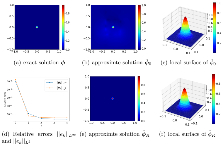
- For two-dimensional Poisson problems with one peak, two peaks, and line singularities, four adaptive iterations bring reported relative $L_\infty$ errors from order $10^{-1}$ down to order $10^{-10}$ at $J_n = 4000$ features per subdomain.
- Because the method is mesh-free, the same gradient-guided resampling applies in complex geometries where constructing and refining a mesh is expensive.
- For the moving-peak heat equation, the adaptation tracks the peak from time step to time step, keeping final-time relative errors near $10^{-7}$ with $\alpha = 1000$.
- For the one-dimensional Burgers equation with $\epsilon = 0.006$, AFCM combined with Picard iteration reaches relative errors near $10^{-6}$ for $J_n = 4000$, showing the mechanism is not limited to linear problems.
- The paper claims the method is more accurate and more efficient than the finite element method on these benchmarks, without needing the singularity location in advance.
Reading between the lines
- Since the monitor is the gradient of the current approximation rather than the true solution, the same loop could be run to convergence as a self-stopping criterion when the exact solution is unknown: stop when two successive adapted solutions barely change, which the examples suggest happens by $K=4$.
- The anchoring constraint, which forces each hyperplane through a sampled point, behaves like a one-step moving-mesh equidistribution rule; if a convergence theory exists for the moving-mesh analogy, it may transfer and yield a priori error estimates for AFCM.
- A testable extension is to replace the gradient monitor by a residual-based monitor for solutions with oscillations instead of steep fronts, where large gradients are not the limiting feature.
- The experiments leave open how sensitive the method is to the constants $c_1$ and $c_2$ and to the initial fit's ability to see the singularity; this could be probed by starting from a deliberately too-coarse initial approximation.
Editorial analysis
A structured set of objections, weighed in public.
Referee Report
Summary. The paper proposes the Adaptive Feature Capture Method (AFCM), an iterative extension of the Random Feature Method (RFM) for PDEs with near-singular or steep-gradient solutions. At each adaptation step, the method uses the gradient norm of the current approximate solution as a monitor function to resample partition hyperplanes and collocation points, and to rescale the shape parameters of the random feature functions. The algorithm is tested on five manufactured problems: two-dimensional Poisson equations with one or two Gaussian peaks, two Poisson equations with line-type ridges of different sharpness, a one-dimensional Burgers equation with a moving front, and a two-dimensional heat equation with a moving peak. In all cases, the relative errors after K=4 adaptation iterations are several orders of magnitude smaller than at the initial iteration. The paper claims that AFCM achieves this accuracy without prior knowledge of the singularity location, without additional computational overhead, and with better accuracy and efficiency than the traditional finite element method.
Significance. If the central claims are correct, AFCM would be a simple, mesh-free adaptive strategy that substantially improves the practical accuracy of the random feature method on steep-gradient problems. The numerical evidence for the core mechanism is strong: the k=0 versus k=4 error reductions are consistent across five different PDEs and several feature counts, and the errors improve monotonically as Jn increases in most cases. The use of manufactured exact solutions makes the reported error norms meaningful. However, the advertised comparison with the finite element method is not supported by any FEM experiment, and the claim of no additional computational overhead is contradicted by the repeated least-squares solves and gradient evaluations in Algorithm 1. In addition, the monitor function inherits the limitations of the initial approximation, a regime that is not stress-tested in the paper. The contribution is therefore a promising numerical heuristic whose scope is currently broader than the evidence supports.
major comments (4)
- [Abstract; Section 5] The claim that AFCM performs "better than the traditional finite element method" appears in the abstract and in Section 5, but no FEM experiment, comparison table, or FEM error or cost data is reported anywhere in Section 4. This is a load-bearing advertised result and should be either removed or substantiated with a head-to-head comparison on the same examples, reporting both accuracy and wall-clock time.
- [Section 3, Eq. (17)] The sampling density p(x) is built from the gradient norm of the current approximate solution. If the k=0 RFM solution does not already contain a visible peak or ridge, the adapted features are placed where the approximate gradient is large, which may be far from the true steep layer. All manufactured solutions in Section 4 are smooth Gaussians or tanh profiles whose peaks are already resolved, albeit inaccurately, at k=0, as shown by the figures and by the k=0 errors in Tables 2-6. The paper does not test the regime where the feature is initially invisible, for example a much narrower layer, a genuinely discontinuous solution, or a much smaller initial Jn. Without such a test, the claim of resolving near-singular solutions "without prior information" is not supported.
- [Section 3, Algorithm 1; Section 4] The statement that AFCM achieves higher resolution "without increasing computational overhead" is not supported by the experiments. Algorithm 1 solves K+1 least-squares systems and, at each iteration, evaluates gradients on up to m = 1.26e6 points and performs weighted sampling. The tables compare k=0 with k=4 but report no wall-clock time, no flop counts, and no comparison with a one-shot RFM using the same total feature budget or with uniform refinement. The efficiency claim needs either a quantitative cost comparison or a rewording to something like "without increasing the number of feature functions."
- [Section 3, Algorithm 1; Section 5] The text in Section 5 says the adaptation repeats until no further improvement in the approximate solution can be made, but Algorithm 1 fixes the number of iterations K and all experiments use K=4. No stopping criterion is given, and no iteration-history table shows that K=4 is sufficient or that later iterations do not degrade the solution. The paper should either specify a concrete stopping criterion, such as a threshold on the relative change between successive approximations, or present the error as a function of k for several more iterations.
minor comments (8)
- [Sections 4.3 and 4.4] Both subsections are titled "Two-Dimensional Poisson Equation with Line Singularity"; rename the second one to distinguish the sharper line, for example "Sharper Line Singularity."
- [Eq. (21)] The relative L2 error norm is not defined on a discrete set; please specify the quadrature rule or the sampling grid used to evaluate the norms reported in the tables.
- [Eq. (7)] The loss function has unclear notation: the subscripts on lambda_n,q and the summation ranges are garbled in the typeset version. Please rewrite the equation cleanly.
- [Table 7] The table header says T = 1.0 while the text and the table body report T = 2.0; please correct this inconsistency.
- [Figures 13 and 14] The captions say "t = 0.2 (left), 1.0 (middle), 2.0 (left)"; the last entry should read "2.0 (right)."
- [Figures 3, 5, 7, 9, 11, 13, 14] The phrase "approximte solution" is a typo for "approximate solution" in the figure captions.
- [Section 4.5] The sentence "We utilize Picard's iterative methods to handle nonlinearity address nonlinearity" contains a duplicated phrase; also specify the Picard tolerance or the number of inner iterations used.
- [Abstract and Section 5] The abstract and conclusions claim applicability to "complex geometries," but all experiments are on rectangles or a square; either add a complex-geometry example, such as an L-shaped or circular domain, or remove this claim.
Circularity Check
No significant circularity: the gradient-monitor feedback is an iterative solve, not a fitted prediction; the only self-citation is background.
full rationale
The method's derivation chain is self-contained in the relevant sense. The k=0 solution is obtained by solving the RFM least-squares problem (7)-(8) with random features, and the adaptation in Eqs. (17)-(19) uses the current gradient norm only as a sampling density before re-solving the same least-squares problem. The exact solution never enters as a fitted parameter; the reported 'predictions' are relative errors on manufactured solutions (Tables 2-7) whose source terms and boundary conditions are derived from the exact solutions, which is external benchmarking rather than circular reasoning. The gradient monitor is a standard iterative moving-mesh feedback device, not a quantity determined by the target answer. If the initial solution misses a sharp feature, later iterations would inherit that blind spot, but no experiment starts in that regime; this is a robustness limitation, not a circularity. The only self-citation is Ref. [37] (Ren & Wang, sharing a coauthor with the present paper), used in the introduction's background sentence on moving mesh methods; it is not load-bearing and no uniqueness or correctness claim is imported from it. Statements such as 'better than the traditional finite element method' and 'repeats this adaptation process until no further improvement' are not substantiated by the displayed experiments (no FEM comparison table, fixed K=4), but those are completeness and correctness concerns, not circularity. Overall, no circular step reduces a claimed result to an input by construction.
Assumptions & free parameters
free parameters (6)
- c1 =
0.01
- c2 =
50
- correlation length eta =
0.5
- initial shape parameter gamma_n =
2.0, 2.6, 2.8, 3.4 for Jn=1500, 2000, 3000, 4000
- adaptation iterations K =
4
- density bandwidth tau =
0.2
assumptions (4)
- domain assumption Gradient norm of the approximate solution is a reliable monitor of where the exact solution has high gradients.
- standard math Random features with partition of unity can represent the target near-singular solution if enough features are placed locally.
- domain assumption The linear least-squares collocation system remains well conditioned after adaptive resampling.
- domain assumption Picard iteration converges for the nonlinear Burgers example.
Cite this review
Pith. "Pith review of Adaptive feature capture method for solving partial differential equations with near singular solutions." pith.science (2026). https://pith.science/paper/EUMNXJOU
@misc{pith2026250712941,
  author       = {Pith},
  title        = {Pith review of: Adaptive feature capture method for solving partial differential equations with near singular solutions},
  year         = {2026},
  howpublished = {\url{https://pith.science/paper/EUMNXJOU}},
  note         = {Machine review of arXiv:2507.12941}
}
read the original abstract
Partial differential equations (PDEs) with near singular solutions pose significant challenges for traditional numerical methods, particularly in complex geometries where mesh generation and adaptive refinement become computationally expensive. Although deep-learning-based approaches, such as Physics-Informed Neural Networks (PINNs) and the Random Feature Method (RFM), offer mesh-free alternatives, they often lack adaptive resolution in critical regions, limiting their accuracy for solutions with steep gradients or singularities. In this work, we propose the Adaptive Feature Capture Method (AFCM), a novel machine learning framework that adaptively redistributes neurons and collocation points in high-gradient regions to enhance local expressive power. Inspired by adaptive moving mesh techniques, AFCM uses the gradient norm of an approximate solution as a monitor function to guide the reinitialization of feature function parameters. This ensures that partition hyperplanes and collocation points cluster where they are most needed, achieving higher resolution without increasing computational overhead. The AFCM extends the capabilities of RFM to handle PDEs with near-singular solutions while preserving its mesh-free efficiency. Numerical experiments demonstrate the method's effectiveness in accurately resolving near-singular problems with a performance that is better than that of the traditional finite element method in terms of accuracy and efficiency. AFCM offers a robust and scalable approach to solving challenging PDEs in scientific and engineering applications.
Figures


Figures from the paper (12 more)


Forward citations
Cited by 1 Pith paper
-
A Morphology-Adaptive Random Feature Method for Inverse Source Problem of the Helmholtz Equation
The two-phase Morphology-Adaptive Random Feature Method solves the multi-frequency Helmholtz inverse source problem by adaptive quadrature plus morphology-matched basis functions, reaching 1.3–16% relative l2 errors o...
Reference graph
Works this paper leans on
-
[1]
L. Debnath, L. Debnath, Nonlinear partial differential equations for sci- entists and engineers, Vol. 2, Springer, 2005
work page 2005
- [2]
-
[3]
A. W. Leung, Systems of nonlinear partial differential equations: appli- cations to biology and engineering, Vol. 49, Springer Science & Business Media, 2013
work page 2013
-
[4]
R. J. LeVeque, Finite difference methods for ordinary and partial dif- ferential equations: steady-state and time-dependent problems, SIAM, 2007
work page 2007
-
[5]
F. Moukalled, L. Mangani, M. Darwish, F. Moukalled, L. Mangani, M. Darwish, The Finite Volume Method, Springer, 2016
work page 2016
-
[6]
Thom´ ee, Galerkin Finite Element Methods for Parabolic Problems, Vol
V. Thom´ ee, Galerkin Finite Element Methods for Parabolic Problems, Vol. 25, Springer Science & Business Media, 2007
work page 2007
-
[7]
O. C. Zienkiewicz, R. L. Taylor, J. Zhu, The Finite Element Method: Its Basis and Fundamentals, Elsevier, 2005
work page 2005
-
[8]
S. Rajendran, A technique to develop mesh-distortion immune finite elements, Computer Methods in Applied Mechanics and Engineering 199 (17-20) (2010) 1044–1063
work page 2010
Show all 40 references
-
[9]
Blazek, Computational fluid dynamics: principles and applications, Butterworth-Heinemann, 2015
J. Blazek, Computational fluid dynamics: principles and applications, Butterworth-Heinemann, 2015
2015
-
[10]
Goodfellow, Y
I. Goodfellow, Y. Bengio, A. Courville, Deep learning, MIT press, 2016
2016
-
[11]
Cybenko, Approximation by superpositions of a sigmoidal function, Mathematics of control, signals and systems 2 (4) (1989) 303–314
G. Cybenko, Approximation by superpositions of a sigmoidal function, Mathematics of control, signals and systems 2 (4) (1989) 303–314
1989
-
[12]
W. E, J. Han, A. Jentzen, Deep Learning-Based Numerical Methods for High-Dimensional Parabolic Partial Differential Equations and Back- ward Stochastic Differential Equations, Communications in Mathemat- ics and Statistics 5 (5) (2017) 349–380
2017
-
[13]
J. Han, A. Jentzen, W. E, Solving high-dimensional partial differential equations using deep learning, Proceedings of the National Academy of Sciences 115 (34) (2018) 8505–8510
2018
-
[14]
W. E, B. Yu, The Deep Ritz Method: A Deep Learning-Based Nu- merical Algorithm for Solving Variational Problems, Communications in Mathematics and Statistics 6 (2018) 1–12. 33
2018
-
[15]
Sirignano, K
J. Sirignano, K. Spiliopoulos, DGM: A deep learning algorithm for solv- ing partial differential equations, Journal of computational physics 375 (2018) 1339–1364
2018
-
[16]
Y. Zang, G. Bao, X. Ye, H. Zhou, Weak adversarial networks for high- dimensional partial differential equations, Journal of Computational Physics 411 (2020) 109409
2020
-
[17]
Raissi, P
M. Raissi, P. Perdikaris, G. E. Karniadakis, Physics-informed neural networks: A deep learning framework for solving forward and inverse problems involving nonlinear partial differential equations, Journal of Computational physics 378 (2019) 686–707
2019
-
[18]
W. E, J. Han, A. Jentzen, Algorithms for solving high dimensional PDEs: from nonlinear Monte Carlo to machine learning, Nonlinearity 35 (1) (2021) 278
2021
-
[19]
Z. Lin, Y. Wang, H. Xie, Adaptive neural network subspace method for solving partial differential equations with high accuracy, arXiv preprint arXiv:2412.02586 (2024)
2024 arXiv
-
[20]
Zhang, W
W. Zhang, W. Suo, J. Song, W. Cao, Physics Informed Neural Net- works (pinns) as intelligent computing technique for solving partial dif- ferential equations: Limitation and future prospects, arXiv preprint arXiv:2411.18240 (2024)
2024 arXiv
-
[21]
Huang, Q.-Y
G.-B. Huang, Q.-Y. Zhu, C.-K. Siew, Extreme learning machine: Theory and applications, Neurocomputing 70 (1-3) (2006) 489–501
2006
-
[22]
R. M. Neal, Bayesian learning for neural networks, Vol. 118, Springer Science & Business Media, 2012
2012
-
[23]
Rahimi, B
A. Rahimi, B. Recht, Random features for large-scale kernel machines, in: Proceedings of the 21st International Conference on Neural Informa- tion Processing Systems, Curran Associates Inc., 2007, p. 1177–1184
2007
-
[24]
Huang, G.-B
G. Huang, G.-B. Huang, S. Song, K. You, Trends in extreme learning machines: A review, Neural Networks 61 (2015) 32–48
2015
-
[25]
J. Chen, X. Chi, Z. Yang, et al., Bridging Traditional and Machine Learning-Based Algorithms for Solving PDEs: The Random Feature Method, J Mach Learn 1 (2022) 268–98. 34
2022
-
[26]
J. Chen, Y. Luo, et al., The Random Feature Method for Time- dependent Problems, arXiv preprint arXiv:2304.06913 (2023)
2023 arXiv
-
[27]
Huang, L
G.-B. Huang, L. Chen, C.-K. Siew, Universal Approximation using In- cremental Constructive Feedforward Networks with Random Hidden Nodes, IEEE transactions on neural networks 17 (4) (2006) 879–892
2006
-
[28]
Dwivedi, B
V. Dwivedi, B. Srinivasan, Physics Informed Extreme Learning Machine (PIELM)–A rapid method for the numerical solution of partial differen- tial equations, Neurocomputing 391 (2020) 96–118
2020
-
[29]
Calabr` o, G
F. Calabr` o, G. Fabiani, C. Siettos, Extreme learning machine colloca- tion for the numerical solution of elliptic PDEs with sharp gradients, Computer Methods in Applied Mechanics and Engineering 387 (2021) 114188
2021
-
[30]
S. Dong, Z. Li, Local extreme learning machines and domain decom- position for solving linear and nonlinear partial differential equations, Computer Methods in Applied Mechanics and Engineering 387 (2021) 114129
2021
-
[31]
Fabiani, F
G. Fabiani, F. Calabr` o, L. Russo, C. Siettos, Numerical solution and bifurcation analysis of nonlinear partial differential equations with ex- treme learning machines, Journal of Scientific Computing 89 (2) (2021) 44
2021
-
[32]
Y. Yang, M. Hou, J. Luo, A novel improved extreme learning machine algorithm in solving ordinary differential equations by Legendre neural network methods, Advances in Difference Equations 2018 (1) (2018) 469
2018
-
[33]
Y. Wang, S. Dong, An extreme learning machine-based method for com- putational pdes in higher dimensions, Computer Methods in Applied Mechanics and Engineering 418 (2024) 116578
2024
-
[34]
H. Dang, F. Wang, S. Jiang, Adaptive growing randomized neu- ral networks for solving partial differential equations, arXiv preprint arXiv:2408.17225 (2024)
2024
-
[35]
J. Sun, S. Dong, F. Wang, Local randomized neural networks with dis- continuous Galerkin methods for partial differential equations, Journal of Computational and Applied Mathematics 445 (2024) 115830. 35
2024
-
[36]
Huang, H
J. Huang, H. Wu, T. Zhou, Adaptive neural network basis methods for partial differential equations with low-regular solutions, arXiv preprint arXiv:2411.01998 (2024)
2024 arXiv
-
[37]
W. Ren, X. Wang, An iterative grid redistribution method for singular problems in multiple dimensions, Journal of Computational Physics 159 (2000) 246–273
2000
-
[38]
Huang, R
W. Huang, R. D. Russell, Adaptive Moving Mesh Method, Springer, 2010
2010
-
[39]
J. I. Ramos, Picard’s iterative method for nonlinear advection–reaction– diffusion equations, Applied Mathematics and Computation 215 (4) (2009) 1526–1536
2009
-
[40]
Zhang, F
Z. Zhang, F. Bao, L. Ju, G. Zhang, Transferable Neural Networks for Partial Differential Equations, Journal of Scientific Computing 99 (1) (2024) 2. 36
2024
Reviewed August 6, 2026 · model on record in the stance chip above.
Discussion (0). Continue with ORCID to comment.