REVIEW 4 major objections 5 minor 36 references
Reduced Subgrid Scale Terms in Three-Dimensional Turbulence
T0 review · 4 major / 5 minor · reviewed 2026-08-06 · deepseek-v4-flash
Pith's one-line read The tau-orthogonal method reduces 3D subgrid closure to six scalar time series, and the stochastic LRS model reproduces long-term turbulence statistics below a tuned Smagorinsky baseline.
desk verdict A clean 3D extension of the tau-orthogonal SGS idea with a cheap stochastic time-series closure; the headline QoI match is partially in-sample, but the paper is honest, reproducible, and deserves a serious referee. read the letter →
The pith
A machine-rendered reading of the paper's core claim, the machinery that carries it, and where it could break.
The reading
What carries the argument
The central object is the tau-orthogonal decomposition of the subgrid term, $m(v,t)=\sum_{i=1}^{N_Q}\tau_i(t)O_i(v)$, where each spatial pattern $O_i$ is built from the weak derivative $V_i$ of the $i$-th scale-aware QoI: $V_i=R_{[l,m]}v$ for banded energy and $V_i=2\nabla\times R_{[l,m]}\omega$ for banded enstrophy. The patterns are constructed to satisfy the orthogonality condition $\int_\Omega V_i\cdot O_j\,dx=0$ for $i\neq j$, so each coefficient $\tau_i$ controls exactly one QoI. The unclosed coefficients are extracted by tracking reference QoI trajectories in a predictor-corrector step and then predicted by the LRS model, a regularized least-squares regression on a history of lagged QoI values plus a multivariate Gaussian residual. This keeps the learning task low-dimensional and independent of spatial resolution, and it couples Fourier-based scale awareness to a staggered-grid solver that operates entirely in physical space.
What would settle it
Run the TO LRS model on a flow whose unresolved dynamics are dominated by something other than the six energy and enstrophy bands, such as scalar mixing or a separating boundary layer, hold out a QoI that tracks that process, and compare its long-term distribution with a tuned eddy-viscosity model; if the held-out statistic drifts more than the baseline does, the six-QoI span assumption is the failure point.
Extended reading notes
Core claim
The paper claims that in three-dimensional large-eddy simulation the subgrid closure can be carried by six scalar time series: energy and enstrophy in three wavenumber bands, rather than by a model of the full subgrid stress tensor. A stochastic linear-regression model with Gaussian residuals, trained on those series via a nudging predictor-corrector procedure, closes the filtered equations stably for 100 time units, reproduces the long-term QoI distributions and the time-averaged energy spectrum, and preserves coherent vortex structures, all with 100 to 1000 parameters. In the isotropic test case its summed Kolmogorov-Smirnov distance sits well below a tuned Smagorinsky baseline. In channel flow the geometry-agnostic model remains stable, captures the mean velocity profile away from the wall, and avoids the small-scale energy buildup seen with the WALE baseline, while underestimating velocity in the few grid points nearest the wall.
Load-bearing premise
The load-bearing premise is that everything the subgrid force does to the large scales shows up in the six banded energy and enstrophy values; a flow whose unresolved dynamics matter through some other statistic would be invisible to this closure.
Editorial extensions
If this is right
- A coarse LES can be closed without ever constructing or learning the full subgrid stress tensor; the closure lives in the history of six scalar QoIs.
- Fourier-scale-aware training statistics can be coupled to a purely physical-space staggered-grid solver, so the method does not require a spectral solver at run time.
- The model extrapolates in time: trained on 10 time units, it runs stably for 100 time units and preserves long-term distributions, spectra, and coherent vortices.
- Performance is robust across a wide band of history lengths; instabilities appear only at zero or very long histories, and light regularization stabilizes data-scarce training at some cost in distribution accuracy.
- In wall-bounded flow the geometry-agnostic model generalizes to a different turbulence regime, matching the mean velocity away from the wall and avoiding the small-scale energy buildup seen with WALE, while underestimating velocity in the few grid points nearest the wall.
Reading between the lines
- Because the model's input space is just six scalars and its parameter count is independent of grid resolution, the same training pipeline should transfer to other integrated observables, such as passive-scalar variance or Reynolds-stress components; that extension is not tested in the paper.
- The five-replica ensemble produced by the stochastic residual could be read as a cheap uncertainty estimate for LES forecasts, though the paper does not analyze whether the ensemble spread is calibrated.
- The near-wall deficit in channel flow suggests the six Fourier-band QoIs carry little information about wall-attached dynamics; adding a wall-normal-aware QoI would be the natural next test of the span assumption.
Editorial analysis
A structured set of objections, weighed in public.
Referee Report
Summary. This paper extends the tau-orthogonal (TO) method for reduced subgrid-scale modeling to three-dimensional turbulent flows. The key step is to replace the high-dimensional SGS closure problem with a low-dimensional one: the SGS forcing is written as a weighted sum of spatial patterns associated with six scale-aware quantities of interest (QoIs), namely kinetic energy and enstrophy in three wavenumber bands. In a predictor-corrector setup, the weights are first extracted by nudging a coarse solver toward reference QoI trajectories obtained from a high-fidelity simulation. A stochastic time-series model (LRS) is then trained to predict the corrected QoIs from lagged QoI values and a Gaussian residual, and is used as a standalone SGS closure. The model is tested in forced homogeneous isotropic turbulence and in turbulent channel flow, and compared with tuned Smagorinsky and WALE models using summed Kolmogorov-Smirnov distances of QoI distributions, kinetic energy spectra, mean velocity profiles, and flow-structure visualizations.
Significance. The contribution is potentially significant. If the validation can be made non-circular, the paper demonstrates that a closure with only 100-1000 parameters, trained on six scalar trajectories, can match or beat classical eddy-viscosity models in two 3D benchmarks while remaining interpretable and cheap. The code and data scripts are publicly available, which is a strong practical advantage. The TO formulation itself is elegant, and the extension from 2D to 3D with scale-aware QoIs is a natural and useful step. The main weaknesses are that the central span assumption (six QoIs suffice) is untested, and the headline metric (KS distance of the six QoI distributions) is computed on the same variables on which the LRS model was trained and, in part, selected. These issues are fixable with additional experiments, so they do not invalidate the approach but do preclude acceptance as is.
major comments (4)
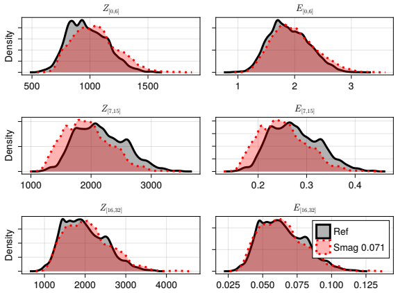
- [Section 4.5, Figure 10; Section 4.7, Figure 15] The hyperparameter scan and the reported performance are based on the same evaluation window. The text states that long-term simulations are used both 'to evaluate the performance' and to 'find suitable hyperparameter settings'. Since the history length, regularization strength, and (in the channel case) the decision to use lambda = 10^-4 are chosen after looking at the summed-KS results on the same 100-time-unit evaluation window, the reported accuracy of the selected LRS configuration is optimistic. The same applies to the Smagorinsky constant tuned in Section 4.4 and the WALE constant in Section 5.5. Please add a clear separation: either state explicitly that Figure 10 is an exploratory scan and report final performance only for a model selected on a different validation period, or use a nested/temporal hold-out (e.g., train on t in [0,10], validate on [10,20], evaluate on [20,100]). Without this, the headline comparison against Smagorinsky is not a strictly out-of-sample test.
- [Section 3.3, Eqs. (26)-(27); Section 4.5, Figures 9-10] The primary success metric is the summed KS distance of the six QoI marginal distributions, which are exactly the quantities whose trajectories are used to train the LRS model. A stable autoregressive model trained on a stationary process will tend to reproduce the marginal distribution of that process, so small KS distances are weak evidence that the TO basis reconstructs the true SGS force rather than merely acting as a fitted stochastic generator. The independent evidence in the paper is limited: Fig. 13 shows a time-averaged spectrum from 10 snapshots of one ensemble member without error bars, and Fig. 21 shows a mean velocity profile (a welcome non-QoI check, but only one). Please add a held-out QoI test (e.g., train on five QoIs and evaluate the sixth), an ablation of the QoI set, or quantitative non-QoI statistics (e.g., SGS dissipation, two-point spectra, or a pointwise comparison with a filtered DNS SGS field) to demonstrate that the learned closure is not just a marginal-distribution fit.
- [Section 3.1, Eq. (23); Section 6] The span assumption is not tested. The method assumes that the six QoIs and the O_i patterns constructed from their weak derivatives span the dynamically relevant part of the SGS force. The paper never varies NQ, never changes the band definitions, and never compares the reconstructed model term m(v,t) with the actual commutator error obtained from filtered DNS snapshots. The near-wall underprediction in the four grid points closest to the wall (Fig. 21) and the future-work statement in Section 6 on 'improving the basis functions' indicate that the span is incomplete at least near solid boundaries. Please include at least one of: (i) a QoI-ablation study, (ii) an a-priori comparison of the learned m against the exact coarse-graining commutator error in a few snapshots, or (iii) a third test case with qualitatively different large-scale anisotropy.
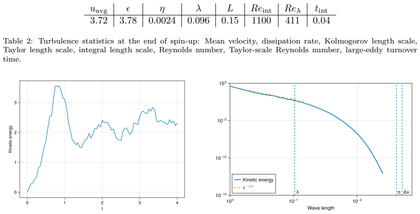
- [Section 4.2, Table 1] The N=512^3 HIT reference is not a full DNS, as the authors state (the Kolmogorov length is limited by the grid size). The LRS model is therefore trained on filtered data that already contain unresolved-scale error, and the reported KS distances are measured against this proxy ground truth. The paper should quantify the resolution deficiency (e.g., k_max*eta, or the fraction of dissipation resolved) and discuss how the residual error in the reference QoIs propagates into the learned closure. If possible, a shorter higher-resolution DNS (e.g., N=1024^3) over a few turnover times would bound the reference error. This is a limitation of the validation rather than a flaw in the method, but it should be addressed for the accuracy claims to stand.
minor comments (5)
- [Table 3] The Smagorinsky row contains eight numerical entries rather than one constant plus six QoI values plus a sum; the layout should be corrected to avoid ambiguity.
- [Section 3.3 vs Section 4.5] The abbreviation for the data-driven noise model is introduced as 'DDM' in Section 3.3 but used as 'DDN' in Section 4.5 and Figure 10; please standardize.
- [Figure 13] The caption should state that the TO LRS curve is from the first ensemble member only and that no error bars or ensemble spread are shown, since the model is stochastic and run-to-run variability matters for the comparison.
- [Appendix B] The phrase 'results in a to low variance' should read 'results in too low variance'.
- [Section 5.3.1] Please clarify how the fractional wavenumber magnitudes in the mirrored wall-normal direction are mapped to the stated integer bands [0,3], [4,10], and [11,17].
Circularity Check
The headline QoI-distribution match is largely a training-fit statement, while the spectrum, structure, and velocity-profile checks are genuine but limited independent evidence.
-
fitted input called prediction
[Section 3.3 (Eqs. 26-27); Section 4.5 (training and Fig. 10)]
"We fit the model to predict the corrected QoIs qn. ... Figure 10 reports the KS-distances between the resulting long-term QoI distributions and the HF reference."
The LRS model's regression target is the corrected QoI vector qn, and the paper's principal validation metric is the long-term distribution of those same qn compared against the HF reference. The training data are sample paths of the reference QoI process; for a stable linear-Gaussian autoregressive model, the fitted conditional mean and residual covariance asymptotically reproduce the stationary marginal of the training process. The summed-KS scores in Figs. 10 and 15 therefore mostly verify that the fitted stochastic process reproduces its own training distribution over a longer horizon, which is a near-in-sample statement for a stationary process rather than an independent test of the SGS closure. The genuinely independent evidence is the time-averaged energy spectrum (Fig.
-
self citation load bearing
[Section 3.1 (Eq. 23 and following text)]
"We choose Tj = Vj. This simple choice of basis functions has given good results in previous work on two-dimensional turbulence [4, 13]."
The ansatz that the spatial patterns Oi are built from weak derivatives Vj (i.e., Tj=Vj) is a load-bearing design choice: it determines the entire structure of the SGS correction. The only justification offered in this paper is that it worked in the authors' own prior work [4,13]. That prior work is not machine-checked or independent, and the present paper does not test alternative basis functions. While the current paper's spectrum, vortex visualizations, and velocity profile provide some empirical support, the QoI-distribution results are partly in-sample, so the basis choice remains justified primarily by self-citation rather than by a derivation or independent validation.
full rationale
The paper's central claim is that the TO LRS model, trained solely on six QoI trajectories, provides a working SGS closure for 3D LES. The validation against long-term QoI distributions is the headline result, but because these QoIs are exactly the quantities the LRS model was trained to reproduce, the distribution match is partly a training-fit statement: a stable linear-Gaussian autoregressive model will tend to reproduce its training marginal in the long run, so the QoI KS scores largely confirm that the fit is self-consistent. The paper's independent evidence consists of the time-averaged energy spectrum (Fig. 13, from 10 snapshots, no error bars), the qualitative vortex-structure plots (Figs. 14 and 22), and the mean velocity profile in channel flow (Fig. 21). These checks are not training targets, but they are limited: they do not test the central span assumption that the six QoIs and their associated patterns Oi capture the dynamically relevant part of the SGS force. The paper itself flags that the high-fidelity HIT simulation is not full DNS (Section 4.2) and that the channel-flow near-wall behavior is deficient (Section 6). Together, these factors make the paper's central claim partially circular: the QoI-distribution success is expected from the fitting procedure, while the genuinely predictive parts are under-supported. However, the paper does include independent external checks (spectrum, structures, velocity profile), and it is not purely a renaming or a pure self-citation chain, so a score of 5 is appropriate rather than higher.
Assumptions & free parameters
free parameters (6)
- LRS regression matrix C =
learned, 100-1000 entries
- Gaussian residual moments mu and Sigma =
learned
- Regularization parameter lambda =
0 (HIT), 1e-4 (channel), 0.01 (Appendix B)
- History length h =
5 (HIT), 5 and 10 (channel)
- Wavenumber band edges =
[0,6],[7,15],[16,32] (HIT); [0,3],[4,10],[11,17] (channel)
- Smagorinsky and WALE constants =
Cs=0.071, Cw=0.53
assumptions (7)
- standard math The incompressible Navier-Stokes equations and the staggered-grid projection solver are an adequate description of the flows studied.
- domain assumption The face-averaging filter preserves the divergence-free property, so the SGS term is divergence-free.
- ad hoc to paper The six selected QoIs and the TO spatial patterns built from their weak derivatives span the relevant SGS correction space.
- domain assumption The QoI process is statistically stationary over the 100 time unit evaluation, so the first 10 time units are representative for training.
- domain assumption The LRS linear model plus Gaussian residual adequately captures the conditional distribution of the corrected QoIs.
- domain assumption The N=512^3 reference simulation is an adequate ground truth for LES validation, despite not being full DNS.
- domain assumption The symmetric mirror extension of the channel flow field yields a valid periodic field for Fourier-based QoIs.
Cite this review
Pith. "Pith review of Reduced Subgrid Scale Terms in Three-Dimensional Turbulence." pith.science (2026). https://pith.science/paper/6YJVKHQF
@misc{pith2026250715539,
  author       = {Pith},
  title        = {Pith review of: Reduced Subgrid Scale Terms in Three-Dimensional Turbulence},
  year         = {2026},
  howpublished = {\url{https://pith.science/paper/6YJVKHQF}},
  note         = {Machine review of arXiv:2507.15539}
}
read the original abstract
Large eddy simulation (LES) has become a central technique for simulating turbulent flows in engineering and applied sciences, offering a compromise between accuracy and computational cost by resolving large scale motions and modeling the effects of smaller, unresolved scales through a subgrid scale (SGS) model. The fidelity and robustness of LES depends critically on the SGS model, particularly in coarse simulations where much of the turbulence spectrum remains unresolved. In this work, we extend the tau-orthogonal (TO) method, a data-driven SGS modeling framework, to three-dimensional turbulent flows. The method reformulates the high-dimensional SGS closure problem as a low-dimensional prediction task focused on scale-aware quantities of interest (QoIs). We extend the model to incorporate QoI-state dependence and temporal correlations by combining regularized least-squares regression with a multivariate Gaussian residual model. This yields a simple yet effective stochastic time-series prediction model (the LRS model), with orders-of-magnitude fewer parameters than typical deep learning approaches which try to directly learn the high-dimensional SGS closure. We demonstrate the effectiveness of the TO LRS model in three-dimensional forced isotropic turbulence and turbulent channel flow. The model achieves accurate long-term QoI distributions, robust performance across hyperparameter settings, and good reproduction of key flow features such as kinetic energy spectra and coherent structures, despite being trained solely on QoI trajectories. Comparisons against classical SGS models, including Smagorinsky and WALE formulations, highlight the TO LRS model's balance of accuracy and computational efficiency.
Figures


Figures from the paper (18 more)




Reference graph
Works this paper leans on
-
[1]
S.D. Agdestein and B. Sanderse. Discretize first, filter next: Learning divergence-consistent closure models for large-eddy simulation. Journal of Computational Physics , 522:113577,
-
[2]
S.D. Agdestein, S. Ciarella, B. Sanderse, and R. Hoekstra. IncompressibleNavierStokes.jl (v3.0.0) [Software]. Zenodo, April 2025. doi: https://doi.org/10.5281/zenodo.15294602. 24
-
[3]
A. Chouippe and M. Uhlmann. Forcing homogeneous turbulence in direct numerical simula- tion of particulate flow with interface resolution and gravity. Physics of Fluids , 27(12), 2015. doi: https://doi.org/10.1063/1.4936274
-
[4]
W.N. Edeling and D.T. Crommelin. Reducing data-driven dynamical subgrid scale models by physical constraints. Computers & Fluids , 201:104470, 2020. doi: https://doi.org/10.1016/j. compfluid.2020.104470
arXiv 2020
-
[5]
S.R. Ephrati. Probabilistic data-driven turbulence closure modeling by assimilating statistics. Journal of Computational Physics , page 114234, 2025. doi: https://doi.org/10.1016/j.jcp. 2025.114234
arXiv 2025
-
[6]
V. Eswaran and S.B. Pope. An examination of forcing in direct numerical simulations of turbu- lence. Computers & Fluids , 16(3):257–278, 1988. doi: https://doi.org/10.1016/0045-7930(88) 90013-8
-
[7]
M. Germano, U. Piomelli, P. Moin, and W.H. Cabot. A dynamic subgrid-scale eddy viscosity model. Physics of Fluids A: Fluid Dynamics , 3(7):1760–1765, 1991. doi: https://doi.org/10. 1063/1.857955
work page 1991
-
[8]
J.M. Gimenez, F.M. S ´ ıvori, A.E. Larreteguy, S.I. Monta˜ no, H.J. Aguerre, N.M. Nigro, and S.R. Idelsohn. A multiscale Pseudo-DNS approach for solving turbulent boundary-layer prob- lems. Computer Methods in Applied Mechanics and Engineering , 437:117804, 2025. doi: https://doi.org/10.1016/j.cma.2025.117804
arXiv 2025
Show all 36 references
-
[9]
Girimaji
S.S. Girimaji. Turbulence closure modeling with machine learning: A foundational physics perspective. New Journal of Physics , 26(7):071201, 2024. doi: 10.1088/1367-2630/ad6689
2024 doi
-
[10]
Gottwald, D.T
G.A. Gottwald, D.T. Crommelin, and C.L.E. Franzke. Stochastic climate theory. In C.L.E. Franzke and T.J. O’Kane, editors,Nonlinear and Stochastic Climate Dynamics, page 209–240. Cambridge University Press, 2017. doi: https://doi.org/10.1017/9781316339251.009
2017 doi
-
[11]
Y. Guan, A. Subel, A. Chattopadhyay, and P. Hassanzadeh. Learning physics-constrained subgrid-scale closures in the small-data regime for stable and accurate LES. Physica D: Nonlinear Phenomena, 443:133568, 2023. doi: https://doi.org/10.1016/j.physd.2022.133568
2023
-
[12]
Guillaumin and L
A.P. Guillaumin and L. Zanna. Stochastic-deep learning parameterization of ocean momen- tum forcing. Journal of Advances in Modeling Earth Systems , 13(9):e2021MS002534, 2021. doi: https://doi.org/10.1029/2021MS002534
2021 doi
-
[13]
Hoekstra, D.T
R. Hoekstra, D.T. Crommelin, and W.N. Edeling. Reduced data-driven turbulence closure for capturing long-term statistics. Computers & Fluids , 285:106469, 2024. ISSN 0045-7930. doi: https://doi.org/10.1016/j.compfluid.2024.106469
2024
-
[14]
Hoekstra, S.D
R. Hoekstra, S.D. Agdestein, S. Ciarella, and B. Sanderse. TO IncompressibleNavierStokes.jl (v0.1) [Software]. Zenodo, July 2025. doi: https://doi.org/10.5281/zenodo.15861632
2025 doi
-
[15]
M. Kurz, P. Offenh¨ auser, and A. Beck. Deep reinforcement learning for turbulence modeling in large eddy simulations. International Journal of Heat and Fluid Flow , 99:109094, 2023. doi: https://doi.org/10.1016/j.ijheatfluidflow.2022.109094
2023
-
[16]
M. Kurz, A. Beck, and B. Sanderse. Harnessing equivariance: Modeling turbulence with graph neural networks. arXiv preprint arXiv:2504.07741 , 2025. doi: https://arxiv.org/abs/ 2504.07741
2025 arXiv
-
[17]
Langford and R.D
J.A. Langford and R.D. Moser. Optimal LES formulations for isotropic turbulence. Journal of fluid mechanics , 398:321–346, 1999. doi: https://doi.org/10.1017/S0022112099006369. 25
1999 doi
-
[18]
Lesieur, O
M. Lesieur, O. M´ etais, and P. Comte. Large-eddy simulations of turbulence . Cambridge university press, 2005. doi: https://doi.org/10.1017/CBO9780511755507
2005 doi
-
[19]
Z. Li, W. Peng, Z. Yuan, and J. Wang. Fourier neural operator approach to large eddy simulation of three-dimensional turbulence. Theoretical and Applied Mechanics Letters , 12 (6):100389, 2022. doi: https://doi.org/10.1016/j.taml.2022.100389
2022
-
[20]
Ling and A
Y. Ling and A. Lozano-Duran. Numerically consistent data-driven subgrid-scale model via data assimilation and machine learning. In AIAA SCITECH 2025 Forum , page 1280, 2025. doi: https://doi.org/10.2514/6.2025-1280
2025 doi
-
[21]
B. List, L. Chen, and N. Thuerey. Learned turbulence modelling with differentiable fluid solvers: physics-based loss functions and optimisation horizons. Journal of Fluid Mechanics , 949:A25, 2022. doi: https://doi.org/10.1017/jfm.2022.738
2022 doi
-
[22]
B. List, L. Chen, K. Bali, and N. Thuerey. Differentiability in unrolled training of neural physics simulators on transient dynamics. Computer Methods in Applied Mechanics and Engineering, 433:117441, 2025. doi: https://doi.org/10.1016/j.cma.2024.117441
2025
-
[23]
B. Liu, H. Yu, H. Huang, N. Liu, and X. Lu. Investigation of nonlocal data-driven methods for subgrid-scale stress modeling in large eddy simulation. AIP Advances, 12(6), 2022. doi: https://doi.org/10.1063/5.0094316
2022 doi
-
[24]
Moin and J
P. Moin and J. Kim. On the numerical solution of time-dependent viscous incompressible fluid flows involving solid boundaries. Journal of computational physics , 35(3):381–392, 1980. doi: https://doi.org/10.1016/0021-9991(80)90076-5
1980 doi
-
[25]
Moser, J
R.D. Moser, J. Kim, and N.N. Mansour. Direct numerical simulation of turbulent channel flow up to Reτ =590. Phys. fluids , 11(4):943–945, 1999. doi: https://doi.org/10.1063/1.869966
1999 doi
-
[26]
Nicoud and F
F. Nicoud and F. Ducros. Subgrid-scale stress modelling based on the square of the velocity gradient tensor. Flow, turbulence and Combustion , 62(3):183–200, 1999. doi: https://doi. org/10.1023/A:1009995426001
1999 doi
-
[27]
Park and H
J. Park and H. Choi. Toward neural-network-based large eddy simulation: Application to turbulent channel flow. Journal of Fluid Mechanics , 914:A16, 2021. doi: https://doi.org/10. 1017/jfm.2020.931
2021
-
[28]
Perezhogin, L
P. Perezhogin, L. Zanna, and C. Fernandez-Granda. Generative data-driven approaches for stochastic subgrid parameterizations in an idealized ocean model. Journal of Advances in Modeling Earth Systems , 15(10):e2023MS003681, 2023. doi: https://doi.org/10.1029/ 2023MS003681
2023
-
[29]
S. Rasp. Coupled online learning as a way to tackle instabilities and biases in neural network parameterizations: General algorithms and Lorenz 96 case study (v1. 0). Geoscientific Model Development, 13(5):2185–2196, 2020. doi: https://doi.org/10.5194/gmd-13-2185-2020
2020 doi
-
[30]
Sanderse, P
B. Sanderse, P. Stinis, R. Maulik, and S.E. Ahmed. Scientific machine learning for closure models in multiscale problems: A review. Foundations of Data Science , 7(1):298–337, 2025. doi: https://doi.org/10.3934/fods.2024043
2025 doi
-
[31]
Saura and T
N. Saura and T. Gomez. Subgrid stress tensor prediction in homogeneous isotropic turbulence using 3D-convolutional neural networks. Preprint at SSRN 4184202 , 2022. doi: https://doi. org/10.2139/ssrn.4184202
2022 doi
-
[32]
Shebalin and S.L
J.V. Shebalin and S.L. Woodruff. Kolmogorov flow in three dimensions. Physics of Fluids , 9 (1):164–170, 1997. doi: https://doi.org/10.1063/1.869159. 26
1997 doi
-
[33]
Smagorinsky
J. Smagorinsky. General circulation experiments with the primitive equations: I. the basic experiment. Monthly weather review , 91(3):99–164, 1963
1963
-
[34]
Van Gastelen, W.N
T. Van Gastelen, W.N. Edeling, and B. Sanderse. Energy-conserving neural network for turbulence closure modeling. Journal of Computational Physics , 508:113003, 2024. doi: https://doi.org/10.1016/j.jcp.2024.113003
2024
-
[35]
Vreman and J.G.M
A.W. Vreman and J.G.M. Kuerten. Comparison of direct numerical simulation databases of turbulent channel flow at Reτ =180. Physics of Fluids , 26(1), 2014. doi: https://doi.org/10. 1063/1.4861064. Appendix A. Quadrature in the F ourier domain Our scale-aware QoIs are based on ...
2014
-
[2025]
doi: https://doi.org/10.1016/j.jcp.2024.113577
2024
Reviewed August 6, 2026 · model on record in the stance chip above.
Discussion (0). Continue with ORCID to comment.