REVIEW 3 major objections 5 minor 87 references
Measuring and modelling the Splash with APOGEE/Gaia and ARTEMIS
T0 review · 3 major / 5 minor · reviewed 2026-08-06 · deepseek-v4-flash
Pith's one-line read The paper argues that Splash-like populations in Milky Way-mass galaxies are ubiquitous and correlate with retrograde accreted mass, so a single massive merger is not required to produce the Milky Way's Splash.
desk verdict A solid abundance study with a provocative simulation-side claim that is currently undercut by an uncalibrated definitional bridge between observed and simulated Splash. read the letter →
The pith
A machine-rendered reading of the paper's core claim, the machinery that carries it, and where it could break.
The reading
What carries the argument
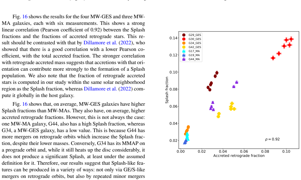
The central object is the Splash itself: a population of old disc stars whose orbits were heated so strongly that they reach high eccentricity and often retrograde motion, defined in the observations as high-$\alpha$ stars with eccentricity $e>0.6$ and in the simulations as in-situ star particles with angular momentum $L_z<0$ at redshift zero. The load-bearing comparison is the correlation of the simulated Splash fraction with the fraction of accreted stars on retrograde orbits, computed within matched solar-neighbourhood annuli ($5<R<11$ kpc, $|Z|<3$ kpc) for four galaxies with a major early merger and three with only minor early accretion. That correlation, rather than any single visual feature, is what lets the paper argue that retrograde orbital orientation is the controlling factor. The observed chemical analysis is carried by two complementary statistics: a per-metallicity-bin comparison of medians with $\chi^2$ values and 1,000 bootstrap resamples, and a $\chi^2$ distribution method that compares Splash abundance trends to 1,000 random disc samples of the same size.
What would settle it
In the ARTEMIS galaxies, compute both eccentricity and angular momentum for every in-situ star particle at $z=0$; if stars with $e>0.6$ turn out to be frequently prograde, or if stars with $L_z<0$ frequently have $e<0.6$, then the observed selection and the simulated definition do not line up, and the $r=0.92$ correlation cannot be assumed to describe the Milky Way's Splash. A second, data-side check would be to measure the Splash fraction in APOGEE outside the solar neighbourhood ($R<5$ kpc) and see whether the simulated dependence of the Splash fraction on radius and height still holds there.
Extended reading notes
Core claim
On the paper's own terms, the discovery is that the Splash is both real and not a unique formation event. In the Milky Way, Splash stars selected by eccentricity $e>0.6$ within the high-$\alpha$ disc differ significantly from the rest of the high-$\alpha$ disc in 12 of 16 abundance ratios: they are richer in $\alpha$ elements, aluminium, and potassium and poorer in manganese, which the paper reads as an older, less chemically enriched population. Yet these differences are not a separate chemical track; they are the extreme end of smooth abundance gradients across eccentricity, meaning the Splash is the heated tail of the old disc. In the ARTEMIS simulations, the same kind of population—defined there as in-situ stars on retrograde orbits at $z=0$—is ubiquitous across Milky Way-mass hosts, whether or not they suffered a major early merger. The decisive variable is retrograde accreted mass: Splash fraction and accreted retrograde fraction correlate with Pearson $r=0.92$, and the minor-merger galaxy G44 out-performs two major-merger galaxies in Splash fraction. The paper concludes that lower-mass retrograde mergers can generate Splash-like populations, so the Milky Way's Splash does not by itself prove a single massive Gaia-Enceladus/Sausage collision.
Load-bearing premise
That the stars the paper identifies as Splash in the Milky Way—high-$\alpha$ stars with eccentricity above 0.6—are the same physical population as the simulated stars it counts as Splash, namely stars born in the host disc that now move on retrograde orbits.
Editorial extensions
If this is right
- A Splash-like population in a galaxy is no longer reliable evidence by itself for a Gaia-Enceladus/Sausage-scale single merger.
- Retrograde accreted mass, not total accreted mass, becomes the predictor to measure when estimating how strongly a galaxy's disc has been heated.
- The Milky Way's Splash could contain contributions from several relatively low-mass retrograde mergers, not just one event, and still show the observed high-alpha, high-Al/K, low-Mn chemistry.
- The calibrated Splash fraction as a function of radius and height can be used to map retrograde accretion histories across the disc and to predict where undiscovered Splash stars might be found.
- Simulations with a major prograde merger but low retrograde accretion predict a weak Splash, implying some Milky Way analogues with a massive early merger would show almost no Splash.
Reading between the lines
- Because the paper uses $L_z<0$ in simulations and $e>0.6$ in observations without direct calibration, a natural next step is to tag ARTEMIS star particles with both quantities simultaneously; if the mapping between the two definitions is loose, the $r=0.92$ correlation would need to be re-derived for the Milky Way's adopted eccentricity cut.
- The paper's simulated [$\mathrm{Mg}/\mathrm{Fe}$]–$L_z$ plane shows a discontinuity at $L_z\sim0$ that is absent in the Milky Way sample; one testable reading is that the Milky Way's Splash is more phase-mixed, or that the observed sample washes out the feature through selection, which could be checked by extending the APOGEE comparison to $R<5$ kpc.
- If retrograde orientation is the controlling variable, then direct measurements of the orbital poles of surviving Milky Way satellites and streams, combined with their masses, could predict the Milky Way's Splash fraction before more stars are observed; the paper's correlation gives a quantitative target for that prediction.
- The chemical pattern—high $[\alpha/\mathrm{Fe}]$, high $[\mathrm{Al},\mathrm{K}/\mathrm{Fe}]$, low $[\mathrm{Mn}/\mathrm{Fe}]$—may serve as a diagnostic of retrograde-heated old disc in other galaxies for which only integrated light is available, though that would require a stellar-population synthesis step the paper does not carry out.
Editorial analysis
A structured set of objections, weighed in public.
Referee Report
Summary. This paper combines APOGEE DR17/Gaia data with ARTEMIS simulations to characterize the Splash. The observational part selects high-[Mg/Fe] giants in the solar neighbourhood and divides them into high-alpha disc (e<0.6) and Splash (e>0.6) samples. Comparing 16 abundance ratios in four metallicity bins, the authors find statistically significant differences, with Splash stars more alpha-enhanced and lower in [Mn/Fe], but also show that these differences vary smoothly with eccentricity. The simulation part defines Splash-like populations in seven ARTEMIS galaxies as in-situ star particles on retrograde orbits (Lz<0), and finds that such populations exist in both GE/S-like and minor-accretion hosts, with a strong correlation (Pearson r=0.92) between the Splash fraction and the fraction of accreted retrograde stars. The authors conclude that retrograde minor mergers can generate Splash-like populations and that orbital orientation matters more than total merger mass.
Significance. The paper's observational analysis is a careful, high-precision chemo-dynamical comparison that extends previous Splash studies to 16 elements. The simulation result, if validated, would be an important step beyond the single-merger narrative: it would imply that Splash-like features are generic to accretion histories and that orbital orientation is a key parameter. Strengths include strict quality cuts, explicit correction for APOGEE log-g abundance systematics, bootstrap-based null chi-squared distributions, and use of a cosmological zoom-in suite with in-situ/accreted labels. However, the central observational-to-simulation link rests on an uncalibrated equivalence between eccentricity and angular-momentum selections, and the simulation sample is small and selected to have high accreted fractions. These caveats are load-bearing for the Splash ubiquity and correlation claims as applied to the Milky Way.
major comments (3)
- [Section 5.1, footnote 3; Sections 5.2-5.4] The manuscript equates the observed Splash definition (e>0.6, Section 2.1) with the simulated definition (in-situ stars with Lz<0, Section 5.2) on the assertion that "Lz correlates very well with eccentricity" (footnote 3). Quantitatively, the two criteria are not equivalent: a star on a highly eccentric prograde orbit has e>0.6 and Lz>0, while a nearly circular retrograde star has Lz<0 and e<0.6. Because every Milky Way comparison in Sections 5.2-5.4 (Fig. 16 correlation, Fig. 13 trend, Fig. 19 ages, and the Fig. 7 versus Fig. 17 confusion maps) uses the simulated Lz<0 definition, the applicability of the main conclusions to the observed Splash depends on this mapping. Please provide a quantitative calibration in ARTEMIS: for the same solar-neighbourhood volume, report the contamination and completeness of the Lz<0 selection relative to an e>0.6 selection (or apply the e>0.6 criterion directly to simulated star particles), and re-derive Fig. 16 and the confusion maps with the matched definition. Without this, the r=0.92 correlation remains an internal simulation result whose connection to the Milky Way Splash is unestablished.
- [Section 5.2, Fig. 16] The headline correlation (Pearson r=0.92) is computed from 42 measurements that are not independent: 6 azimuthal sectors per galaxy, with galaxies strongly clustered in the plane. The significance and confidence interval of r need to account for this clustering, for example by block-bootstrap resampling whole galaxies or using a mixed-effects model. In addition, the two plotted quantities share a common Lz<0 orientation definition at z=0, so a correlation is partly expected if a retrograde merger both deposits retrograde accreted stars and heats the in-situ disc in the same rotational sense. The paper does not control for this shared-orientation effect, for example by comparing with a null that randomizes the sign of Lz, or by partial correlation with the total accreted fraction. Please add such a control before claiming that retrograde orientation specifically drives Splash formation.
- [Section 5.2 and Section 5.4] The conclusion that Splash-like populations are "ubiquitous" (abstract and Section 5.4) is drawn from seven ARTEMIS galaxies, and the paper states that "all systems selected here have high total accreted fractions ... >40%" (Section 5). This selection enriches the sample in accretion-dominated systems and does not justify statements about Milky Way-mass galaxies in general. The ubiquity claim should either be restricted to the selected class of accretion-rich galaxies or supported by a test on a larger, unselected ARTEMIS sample (for example, the full 45-galaxy suite). As written, the claim overreaches the data.
minor comments (5)
- [Sections 5.1 and 6] The text refers to "six simulated galaxies" in two places, but the paper defines and uses seven (G29, G30, G34, G42, G17, G19, G44). Please correct the inconsistency.
- [Fig. 7] The y-axis label reads "Splash fractoin"; this should be "Splash fraction".
- [Fig. 9] All p-values are printed as 0.0; please report them as <0.001 or with a precision consistent with the bootstrap method, since a literal zero probability is not a meaningful statement.
- [Section 5.2] The Splash fraction in simulations is defined as the ratio of in-situ retrograde to prograde stars, while the abstract calls it the "mass fraction of Splash stars". These are different quantities; please clarify which quantity is plotted in Fig. 16 and used in the text.
- [Fig. 13] The Milky Way panel uses -0.6<[Fe/H]<-0.4 while the simulated panels use -1.0<[Fe/H]<-0.8; the text compares the slopes without testing sensitivity to this metallicity choice. A brief check or caveat would be useful.
Circularity Check
The simulated Splash is defined as any in-situ retrograde star, so the 'ubiquitous' claim is partly definitional; the main correlation and observational chemistry are otherwise independent.
-
self definitional
[Section 5.2, definition of Splash fractions; Abstract]
"To compute the Splash fractions, we select all in situ star particles on retrograde orbits (Lz< 0) at redshift 0 and then compute the ratio between the in situ retrograde and prograde populations."
The simulated Splash fraction is defined entirely as the fraction of in-situ stars with Lz<0. Thus the abstract's claim that 'Splash-like populations are ubiquitous' is guaranteed by construction: any galaxy with a kinematically hot disc contains some retrograde in-situ stars, so a non-zero Splash fraction is inevitable. No additional Splash criterion (minimum fraction, eccentricity, chemical distinctness) is imposed. Also, both the simulated Splash and the predictor 'retrograde accreted fraction' are selected by the same sign of Lz, so part of the shared orientation dependence is built into the variables. The r=0.92 correlation is not mathematically forced (the in-situ and accreted sets are disjoint), but the qualitative ubiquity statement is a definitional artefact.
full rationale
The observational analysis (Sections 2-4) is self-contained: the Splash is selected by an eccentricity cut in the high-alpha disc, and the chemical comparisons use bootstrap chi-square tests against the high-alpha population without presupposing the conclusion. The simulation part is largely independent, with two caveats. First, the simulated Splash fraction is defined as the in-situ retrograde fraction, so the abstract's 'ubiquitous' statement is close to a tautology for any galaxy with a hot disc. Second, the observed e>0.6 and simulated Lz<0 criteria are asserted to be equivalent ('Lz correlates very well with eccentricity', with a footnote saying this was verified) but no quantitative calibration is shown; this is a validity threat to the Milky Way comparisons, though not a circular reduction. The key correlation (r=0.92) between in-situ retrograde fraction and accreted retrograde fraction is an empirical relation between disjoint particle sets, and the G44/G34 comparison and [Mg/Fe]-Lz trends provide independent content. Overall, one central qualitative claim is partly definitional, but the main quantitative results do not reduce to their inputs, so a moderate score is appropriate.
Assumptions & free parameters
free parameters (4)
- Splash eccentricity threshold e=0.6 =
e>0.6
- High-alpha selection boundary in [Mg/Fe]-[Fe/H] =
red dashed line (not numerically specified)
- Metallicity comparison window =
-1.1 < [Fe/H] < -0.3
- Per-abundance log g correction polynomials =
2nd-order polynomial coefficients per element
assumptions (4)
- domain assumption APOGEE ASPCAP abundances are reliable after the log-g correction
- domain assumption Galactic orbits computed in the McMillan (2017) potential with the Stäckel fudge are accurate enough for eccentricity and Lz classification
- domain assumption ARTEMIS simulations with WMAP cosmology and subgrid feedback reproduce realistic Milky Way-like galaxies and their merger histories
- ad hoc to paper In-situ retrograde stars in simulations correspond to the observed Splash
Cite this review
Pith. "Pith review of Measuring and modelling the Splash with APOGEE/Gaia and ARTEMIS." pith.science (2026). https://pith.science/paper/HKDVS4CF
@misc{pith2026250715944,
  author       = {Pith},
  title        = {Pith review of: Measuring and modelling the Splash with APOGEE/Gaia and ARTEMIS},
  year         = {2026},
  howpublished = {\url{https://pith.science/paper/HKDVS4CF}},
  note         = {Machine review of arXiv:2507.15944}
}
read the original abstract
Using combined data from SDSS-IV/APOGEE and Gaia, we study the chemo-dynamical properties of the Splash population in comparison with those of the high-alpha disc. We investigate a wide range of abundance ratios, finding that the Splash differs from the high-alpha disc overall. However, these differences result from a smooth variation of chemical compositions as a function of orbital properties. The Splash occupies the high-alpha, high-[Al,K/Fe], and low-[Mn/Fe] end of the high-alpha disk population. In agreement with previous studies, we find that Splash stars are distributed over large heights from the Galactic mid-plane. To further elucidate the relation between the Splash and the high-alpha disk, we turn to simulations. Using a sample of Milky Way-like galaxies with and without major accretion events from the ARTEMIS simulations, we find that Splash-like populations are ubiquitous, though not always resulting from major mergers. Lower mass progenitors can also generate Splash-like features, as long as they are on retrograde orbits. Moreover, we find a strong correlation between the mass fraction of Splash stars and the fraction of retrograde accreted stars in the disk. Some galaxies with minor (retrograde) mergers contain more pronounced Splash populations than others with major, but prograde, mergers. For stars in the high-alpha disks, we also find a decrease in the [alpha/Fe] with increasing orbital angular momentum. This trend is found in hosts with both major or minor mergers. Our results suggest that a number of relatively low-mass mergers on retrograde orbits could result in populations that are qualitatively similar to the Splash.
Figures


Figures from the paper (16 more)




Reference graph
Works this paper leans on
-
[1]
write newline
" write newline "" before.all 'output.state := FUNCTION fin.entry write newline FUNCTION new.block output.state before.all = 'skip after.block 'output.state := if FUNCTION new.sentence output.state after.block = 'skip output.state before.all = 'skip after.sentence 'output.state := if if FUNCTION not #0 #1 if FUNCTION and 'skip pop #0 if FUNCTION or pop #1...
-
[2]
Abdurro'uf et al., 2022, @doi [ ] 10.3847/1538-4365/ac4414 , https://ui.adsabs.harvard.edu/abs/2022ApJS..259...35A 259, 35
-
[3]
Amarante J. A. S., Beraldo e Silva L., Debattista V. P., Smith M. C., 2020, @doi [ ] 10.3847/2041-8213/ab78a4 , https://ui.adsabs.harvard.edu/abs/2020ApJ...891L..30A 891, L30
-
[4]
Andrews B. H., Weinberg D. H., Sch \"o nrich R., Johnson J. A., 2017, @doi [ ] 10.3847/1538-4357/835/2/224 , https://ui.adsabs.harvard.edu/abs/2017ApJ...835..224A 835, 224
-
[5]
Beaton R. L., et al., 2021, @doi [ ] 10.3847/1538-3881/ac260c , https://ui.adsabs.harvard.edu/abs/2021AJ....162..302B 162, 302
-
[6]
Belokurov V., Kravtsov A., 2022, @doi [ ] 10.1093/mnras/stac1267 , https://ui.adsabs.harvard.edu/abs/2022MNRAS.514..689B 514, 689
-
[7]
Belokurov V., et al., 2006, @doi [ ] 10.1086/504797 , https://ui.adsabs.harvard.edu/abs/2006ApJ...642L.137B 642, L137
doi:10.1086/504797 2006
-
[8]
Belokurov V., Erkal D., Evans N. W., Koposov S. E., Deason A. J., 2018, @doi [ ] 10.1093/mnras/sty982 , https://ui.adsabs.harvard.edu/abs/2018MNRAS.478..611B 478, 611
Show all 87 references
-
[9]
L., Fattahi A., Smith M
Belokurov V., Sanders J. L., Fattahi A., Smith M. C., Deason A. J., Evans N. W., Grand R. J. J., 2020, @doi [ ] 10.1093/mnras/staa876 , https://ui.adsabs.harvard.edu/abs/2020MNRAS.494.3880B 494, 3880
2020 doi
-
[10]
Bennett M., Bovy J., 2019, @doi [ ] 10.1093/mnras/sty2813 , https://ui.adsabs.harvard.edu/abs/2019MNRAS.482.1417B 482, 1417
2019 doi
-
[11]
Binney J., 2012, @doi [ ] 10.1111/j.1365-2966.2012.21757.x , https://ui.adsabs.harvard.edu/abs/2012MNRAS.426.1324B 426, 1324
2012
-
[12]
R., et al., 2017, @doi [ ] 10.3847/1538-3881/aa7567 , https://ui.adsabs.harvard.edu/abs/2017AJ....154...28B 154, 28
Blanton M. R., et al., 2017, @doi [ ] 10.3847/1538-3881/aa7567 , https://ui.adsabs.harvard.edu/abs/2017AJ....154...28B 154, 28
2017 doi
-
[13]
F., Kere s D., 2017, @doi [ ] 10.3847/1538-4357/aa7d0c , https://ui.adsabs.harvard.edu/abs/2017ApJ...845..101B 845, 101
Bonaca A., Conroy C., Wetzel A., Hopkins P. F., Kere s D., 2017, @doi [ ] 10.3847/1538-4357/aa7d0c , https://ui.adsabs.harvard.edu/abs/2017ApJ...845..101B 845, 101
2017 doi
-
[14]
Bovy J., 2015, @doi [ ] 10.1088/0067-0049/216/2/29 , https://ui.adsabs.harvard.edu/abs/2015ApJS..216...29B 216, 29
2015 doi
-
[15]
S., Vaughan A
Bowen I. S., Vaughan A. H. J., 1973, @doi [ ] 10.1364/AO.12.001430 , https://ui.adsabs.harvard.edu/abs/1973ApOpt..12.1430B 12, 1430
1973 doi
-
[16]
Chandra V., et al., 2024, @doi [ ] 10.3847/1538-4357/ad5b60 , https://ui.adsabs.harvard.edu/abs/2024ApJ...972..112C 972, 112
2024 doi
-
[17]
Ciuc a I., et al., 2023, @doi [ ] 10.1093/mnrasl/slad033 , https://ui.adsabs.harvard.edu/abs/2023MNRAS.tmpL..32C
2023 doi
-
[18]
P., Parry O
Cooper A. P., Parry O. H., Lowing B., Cole S., Frenk C., 2015, @doi [ ] 10.1093/mnras/stv2057 , https://ui.adsabs.harvard.edu/abs/2015MNRAS.454.3185C 454, 3185
2015 doi
-
[19]
Cui X.-Q., et al., 2012, @doi [Research in Astronomy and Astrophysics] 10.1088/1674-4527/12/9/003 , https://ui.adsabs.harvard.edu/abs/2012RAA....12.1197C 12, 1197
2012 doi
-
[20]
Das P., Hawkins K., Jofr \'e P., 2020, @doi [ ] 10.1093/mnras/stz3537 , https://ui.adsabs.harvard.edu/abs/2020MNRAS.493.5195D 493, 5195
2020 doi
-
[21]
D., Katz D., Khoperskov S., Snaith O
Di Matteo P., Haywood M., Lehnert M. D., Katz D., Khoperskov S., Snaith O. N., G \'o mez A., Robichon N., 2019, @doi [ ] 10.1051/0004-6361/201834929 , https://ui.adsabs.harvard.edu/abs/2019A&A...632A...4D 632, A4
2019 doi
-
[22]
M., Belokurov V., Font A
Dillamore A. M., Belokurov V., Font A. S., McCarthy I. G., 2022, @doi [ ] 10.1093/mnras/stac1038 , https://ui.adsabs.harvard.edu/abs/2022MNRAS.513.1867D 513, 1867
2022 doi
-
[23]
M., Belokurov V., Evans N
Dillamore A. M., Belokurov V., Evans N. W., Davies E. Y., 2023, @doi [ ] 10.1093/mnras/stad2136 , https://ui.adsabs.harvard.edu/abs/2023MNRAS.524.3596D 524, 3596
2023 doi
-
[24]
M., Belokurov V., Kravtsov A., Font A
Dillamore A. M., Belokurov V., Kravtsov A., Font A. S., 2024, @doi [ ] 10.1093/mnras/stad3369 , https://ui.adsabs.harvard.edu/abs/2024MNRAS.527.7070D 527, 7070
2024 doi
-
[25]
W., Rix H.-W., Ness M
Eilers A.-C., Hogg D. W., Rix H.-W., Ness M. K., Price-Whelan A. M., M \'e sz \'a ros S., Nitschelm C., 2022, @doi [ ] 10.3847/1538-4357/ac54ad , https://ui.adsabs.harvard.edu/abs/2022ApJ...928...23E 928, 23
2022 doi
-
[26]
Fernandes L., et al., 2023, @doi [ ] 10.1093/mnras/stac3543 , https://ui.adsabs.harvard.edu/abs/2023MNRAS.519.3611F 519, 3611
2023 doi
-
[27]
S., et al., 2020, @doi [ ] 10.1093/mnras/staa2463 , https://ui.adsabs.harvard.edu/abs/2020MNRAS.498.1765F 498, 1765
Font A. S., et al., 2020, @doi [ ] 10.1093/mnras/staa2463 , https://ui.adsabs.harvard.edu/abs/2020MNRAS.498.1765F 498, 1765
2020 doi
-
[28]
S., McCarthy I
Font A. S., McCarthy I. G., Belokurov V., 2021, @doi [ ] 10.1093/mnras/stab1332 , https://ui.adsabs.harvard.edu/abs/2021MNRAS.505..783F 505, 783
2021 doi
-
[29]
S., McCarthy I
Font A. S., McCarthy I. G., Belokurov V., Brown S. T., Stafford S. G., 2022, @doi [ ] 10.1093/mnras/stac183 , https://ui.adsabs.harvard.edu/abs/2022MNRAS.511.1544F 511, 1544
2022 doi
-
[30]
GRAVITY Collaboration et al., 2019, @doi [ ] 10.1051/0004-6361/201935656 , https://ui.adsabs.harvard.edu/abs/2019A&A...625L..10G 625, L10
2019 doi
-
[31]
Gaia Collaboration et al., 2018, @doi [ ] 10.1051/0004-6361/201833051 , https://ui.adsabs.harvard.edu/abs/2018A&A...616A...1G 616, A1
2018 doi
-
[32]
Gaia Collaboration et al., 2021, @doi [ ] 10.1051/0004-6361/202039657 , https://ui.adsabs.harvard.edu/abs/2021A&A...649A...1G 649, A1
2021 doi
-
[33]
J., Brook C
Gallart C., Bernard E. J., Brook C. B., Ruiz-Lara T., Cassisi S., Hill V., Monelli M., 2019, @doi [Nature Astronomy] 10.1038/s41550-019-0829-5 , https://ui.adsabs.harvard.edu/abs/2019NatAs...3..932G 3, 932
2019 doi
-
[34]
E., et al., 2016, @doi [ ] 10.3847/0004-6256/151/6/144 , https://ui.adsabs.harvard.edu/abs/2016AJ....151..144G 151, 144
Garc \' a P \'e rez A. E., et al., 2016, @doi [ ] 10.3847/0004-6256/151/6/144 , https://ui.adsabs.harvard.edu/abs/2016AJ....151..144G 151, 144
2016 doi
-
[35]
Grand R. J. J., et al., 2017, @doi [ ] 10.1093/mnras/stx071 , https://ui.adsabs.harvard.edu/abs/2017MNRAS.467..179G 467, 179
2017 doi
-
[36]
Grand R. J. J., et al., 2018, @doi [ ] 10.1093/mnras/sty2403 , https://ui.adsabs.harvard.edu/abs/2018MNRAS.481.1726G 481, 1726
2018 doi
-
[37]
Grand R. J. J., et al., 2020, @doi [ ] 10.1093/mnras/staa2057 , https://ui.adsabs.harvard.edu/abs/2020MNRAS.497.1603G 497, 1603
2020 doi
-
[38]
Graur O., et al., 2014, @doi [ ] 10.1088/0004-637X/783/1/28 , https://ui.adsabs.harvard.edu/abs/2014ApJ...783...28G 783, 28
2014 doi
-
[39]
E., et al., 2006, @doi [ ] 10.1086/500975 , https://ui.adsabs.harvard.edu/abs/2006AJ....131.2332G 131, 2332
Gunn J. E., et al., 2006, @doi [ ] 10.1086/500975 , https://ui.adsabs.harvard.edu/abs/2006AJ....131.2332G 131, 2332
2006 doi
-
[40]
Hasselquist S., et al., 2021, @doi [ ] 10.3847/1538-4357/ac25f9 , https://ui.adsabs.harvard.edu/abs/2021ApJ...923..172H 923, 172
2021 doi
-
[41]
Hawkins K., Jofr \'e P., Masseron T., Gilmore G., 2015, @doi [ ] 10.1093/mnras/stv1586 , https://ui.adsabs.harvard.edu/abs/2015MNRAS.453..758H 453, 758
2015 doi
-
[42]
R., et al., 2015, @doi [ ] 10.1088/0004-637X/808/2/132 , https://ui.adsabs.harvard.edu/abs/2015ApJ...808..132H 808, 132
Hayden M. R., et al., 2015, @doi [ ] 10.1088/0004-637X/808/2/132 , https://ui.adsabs.harvard.edu/abs/2015ApJ...808..132H 808, 132
2015 doi
-
[43]
D., Snaith O., Khoperskov S., G \'o mez A., 2018, @doi [ ] 10.3847/1538-4357/aad235 , https://ui.adsabs.harvard.edu/abs/2018ApJ...863..113H 863, 113
Haywood M., Di Matteo P., Lehnert M. D., Snaith O., Khoperskov S., G \'o mez A., 2018, @doi [ ] 10.3847/1538-4357/aad235 , https://ui.adsabs.harvard.edu/abs/2018ApJ...863..113H 863, 113
2018 doi
-
[44]
H., Massari D., Veljanoski J., Brown A
Helmi A., Babusiaux C., Koppelman H. H., Massari D., Veljanoski J., Brown A. G. A., 2018, @doi [ ] 10.1038/s41586-018-0625-x , https://ui.adsabs.harvard.edu/abs/2018Natur.563...85H 563, 85
2018 doi
-
[45]
A., et al., 2015, @doi [ ] 10.1088/0004-6256/150/5/148 , https://ui.adsabs.harvard.edu/abs/2015AJ....150..148H 150, 148
Holtzman J. A., et al., 2015, @doi [ ] 10.1088/0004-6256/150/5/148 , https://ui.adsabs.harvard.edu/abs/2015AJ....150..148H 150, 148
2015 doi
-
[46]
A., et al., 2018, @doi [ ] 10.3847/1538-3881/aad4f9 , https://ui.adsabs.harvard.edu/abs/2018AJ....156..125H 156, 125
Holtzman J. A., et al., 2018, @doi [ ] 10.3847/1538-3881/aad4f9 , https://ui.adsabs.harvard.edu/abs/2018AJ....156..125H 156, 125
2018 doi
-
[47]
Horta D., et al., 2021, @doi [ ] 10.1093/mnras/staa2987 , https://ui.adsabs.harvard.edu/abs/2021MNRAS.500.1385H 500, 1385
2021 doi
-
[48]
Horta D., et al., 2023, @doi [ ] 10.1093/mnras/stac3179 , https://ui.adsabs.harvard.edu/abs/2023MNRAS.520.5671H 520, 5671
2023 doi
-
[49]
L., Ness M
Horta D., Lu Y. L., Ness M. K., Lisanti M., Price-Whelan A. M., 2024, @doi [ ] 10.3847/1538-4357/ad58de , https://ui.adsabs.harvard.edu/abs/2024ApJ...971..170H 971, 170
2024 doi
-
[50]
R., Thielemann F.-K., 1999, @doi [ ] 10.1086/313278 , https://ui.adsabs.harvard.edu/abs/1999ApJS..125..439I 125, 439
Iwamoto K., Brachwitz F., Nomoto K., Kishimoto N., Umeda H., Hix W. R., Thielemann F.-K., 1999, @doi [ ] 10.1086/313278 , https://ui.adsabs.harvard.edu/abs/1999ApJS..125..439I 125, 439
1999 doi
-
[51]
C., Cole S., Frenk C
Jiang L., Helly J. C., Cole S., Frenk C. S., 2014, @doi [ ] 10.1093/mnras/stu390 , https://ui.adsabs.harvard.edu/abs/2014MNRAS.440.2115J 440, 2115
2014 doi
-
[52]
J \"o nsson H., et al., 2020, @doi [ ] 10.3847/1538-3881/aba592 , https://ui.adsabs.harvard.edu/abs/2020AJ....160..120J 160, 120
2020 doi
-
[54]
Lane J. M. M., Bovy J., Mackereth J. T., 2022, @doi [ ] 10.1093/mnras/stab3755 , https://ui.adsabs.harvard.edu/abs/2022MNRAS.510.5119L 510, 5119
2022 doi
-
[55]
S., Kim Y
Lee A., Lee Y. S., Kim Y. K., Beers T. C., An D., 2023, @doi [ ] 10.3847/1538-4357/acb6f5 , https://ui.adsabs.harvard.edu/abs/2023ApJ...945...56L 945, 56
2023 doi
-
[56]
W., Bovy J., 2019, @doi [ ] 10.1093/mnras/stz2245 , https://ui.adsabs.harvard.edu/abs/2019MNRAS.489.2079L 489, 2079
Leung H. W., Bovy J., 2019, @doi [ ] 10.1093/mnras/stz2245 , https://ui.adsabs.harvard.edu/abs/2019MNRAS.489.2079L 489, 2079
2019 doi
-
[57]
T., Bovy J., 2018, @doi [ ] 10.1088/1538-3873/aadcdd , https://ui.adsabs.harvard.edu/abs/2018PASP..130k4501M 130, 114501
Mackereth J. T., Bovy J., 2018, @doi [ ] 10.1088/1538-3873/aadcdd , https://ui.adsabs.harvard.edu/abs/2018PASP..130k4501M 130, 114501
2018 doi
-
[58]
T., et al., 2019, @doi [ ] 10.1093/mnras/sty2955 , https://ui.adsabs.harvard.edu/abs/2019MNRAS.482.3426M 482, 3426
Mackereth J. T., et al., 2019, @doi [ ] 10.1093/mnras/sty2955 , https://ui.adsabs.harvard.edu/abs/2019MNRAS.482.3426M 482, 3426
2019 doi
-
[59]
R., et al., 2017, @doi [ ] 10.3847/1538-3881/aa784d , https://ui.adsabs.harvard.edu/abs/2017AJ....154...94M 154, 94
Majewski S. R., et al., 2017, @doi [ ] 10.3847/1538-3881/aa784d , https://ui.adsabs.harvard.edu/abs/2017AJ....154...94M 154, 94
2017 doi
-
[60]
Martig M., et al., 2016, @doi [ ] 10.1093/mnras/stv2830 , https://ui.adsabs.harvard.edu/abs/2016MNRAS.456.3655M 456, 3655
2016 doi
-
[61]
C., Crain R
Mason A. C., Crain R. A., Schiavon R. P., Weinberg D. H., Pfeffer J., Schaye J., Schaller M., Theuns T., 2024, @doi [ ] 10.1093/mnras/stae1743 , https://ui.adsabs.harvard.edu/abs/2024MNRAS.533..184M 533, 184
2024 doi
-
[62]
G., Font A
McCarthy I. G., Font A. S., Crain R. A., Deason A. J., Schaye J., Theuns T., 2012, @doi [ ] 10.1111/j.1365-2966.2011.20189.x , https://ui.adsabs.harvard.edu/abs/2012MNRAS.420.2245M 420, 2245
2012
-
[63]
J., 2017, @doi [ ] 10.1093/mnras/stw2759 , https://ui.adsabs.harvard.edu/abs/2017MNRAS.465...76M 465, 76
McMillan P. J., 2017, @doi [ ] 10.1093/mnras/stw2759 , https://ui.adsabs.harvard.edu/abs/2017MNRAS.465...76M 465, 76
2017 doi
-
[64]
P., Conroy C., Bonaca A., Johnson B
Naidu R. P., Conroy C., Bonaca A., Johnson B. D., Ting Y.-S., Caldwell N., Zaritsky D., Cargile P. A., 2020, @doi [ ] 10.3847/1538-4357/abaef4 , https://ui.adsabs.harvard.edu/abs/2020ApJ...901...48N 901, 48
2020 doi
-
[65]
L., et al., 2015, @doi [ ] 10.1088/0004-6256/150/6/173 , https://ui.adsabs.harvard.edu/abs/2015AJ....150..173N 150, 173
Nidever D. L., et al., 2015, @doi [ ] 10.1088/0004-6256/150/6/173 , https://ui.adsabs.harvard.edu/abs/2015AJ....150..173N 150, 173
2015 doi
-
[66]
Ortigoza-Urdaneta M., et al., 2023, @doi [ ] 10.1051/0004-6361/202346325 , https://ui.adsabs.harvard.edu/abs/2023A&A...676A.140O 676, A140
2023 doi
- [67]
-
[68]
Ratcliffe B., et al., 2023, @doi [ ] 10.1093/mnras/stad1573 , https://ui.adsabs.harvard.edu/abs/2023MNRAS.525.2208R 525, 2208
2023 doi
-
[69]
J., Brunthaler A., 2020, @doi [ ] 10.3847/1538-4357/ab76cd , https://ui.adsabs.harvard.edu/abs/2020ApJ...892...39R 892, 39
Reid M. J., Brunthaler A., 2020, @doi [ ] 10.3847/1538-4357/ab76cd , https://ui.adsabs.harvard.edu/abs/2020ApJ...892...39R 892, 39
2020 doi
-
[70]
Renzini A., Voli M., 1981, , https://ui.adsabs.harvard.edu/abs/1981A&A....94..175R 94, 175
1981
-
[71]
A., et al., 2021, @doi [ ] 10.3847/1538-3881/ac2cbc , https://ui.adsabs.harvard.edu/abs/2021AJ....162..303S 162, 303
Santana F. A., et al., 2021, @doi [ ] 10.3847/1538-3881/ac2cbc , https://ui.adsabs.harvard.edu/abs/2021AJ....162..303S 162, 303
2021 doi
-
[72]
P., et al., 2017, @doi [ ] 10.1093/mnras/stw2162 , https://ui.adsabs.harvard.edu/abs/2017MNRAS.465..501S 465, 501
Schiavon R. P., et al., 2017, @doi [ ] 10.1093/mnras/stw2162 , https://ui.adsabs.harvard.edu/abs/2017MNRAS.465..501S 465, 501
2017 doi
-
[73]
P., et al., 2024, @doi [ ] 10.1093/mnras/stad3020 , https://ui.adsabs.harvard.edu/abs/2024MNRAS.528.1393S 528, 1393
Schiavon R. P., et al., 2024, @doi [ ] 10.1093/mnras/stad3020 , https://ui.adsabs.harvard.edu/abs/2024MNRAS.528.1393S 528, 1393
2024 doi
-
[74]
Sch \"o nrich R., Binney J., Dehnen W., 2010, @doi [ ] 10.1111/j.1365-2966.2010.16253.x , https://ui.adsabs.harvard.edu/abs/2010MNRAS.403.1829S 403, 1829
2010
-
[75]
R., Bland-Hawthorn J., 2021, @doi [ ] 10.1093/mnras/stab2015 , https://ui.adsabs.harvard.edu/abs/2021MNRAS.507.5882S 507, 5882
Sharma S., Hayden M. R., Bland-Hawthorn J., 2021, @doi [ ] 10.1093/mnras/stab2015 , https://ui.adsabs.harvard.edu/abs/2021MNRAS.507.5882S 507, 5882
2021 doi
-
[76]
Siess L., 2010, @doi [ ] 10.1051/0004-6361/200913556 , https://ui.adsabs.harvard.edu/abs/2010A&A...512A..10S 512, A10
2010 doi
-
[77]
Springel V., 2005, @doi [ ] 10.1111/j.1365-2966.2005.09655.x , https://ui.adsabs.harvard.edu/abs/2005MNRAS.364.1105S 364, 1105
2005
-
[78]
Springel V., White S. D. M., Tormen G., Kauffmann G., 2001, @doi [ ] 10.1046/j.1365-8711.2001.04912.x , https://ui.adsabs.harvard.edu/abs/2001MNRAS.328..726S 328, 726
2001
-
[79]
Srisawat C., et al., 2013, @doi [ ] 10.1093/mnras/stt1545 , https://ui.adsabs.harvard.edu/abs/2013MNRAS.436..150S 436, 150
2013 doi
-
[80]
J., et al., 2022, @doi [ ] 10.1093/mnras/stac968 , https://ui.adsabs.harvard.edu/abs/2022MNRAS.513.3429T 513, 3429
Taylor D. J., et al., 2022, @doi [ ] 10.1093/mnras/stac968 , https://ui.adsabs.harvard.edu/abs/2022MNRAS.513.3429T 513, 3429
2022 doi
-
[81]
Tolstoy E., Hill V., Tosi M., 2009, @doi [ ] 10.1146/annurev-astro-082708-101650 , https://ui.adsabs.harvard.edu/abs/2009ARA&A..47..371T 47, 371
2009 doi
-
[82]
H., et al., 2022, @doi [ ] 10.3847/1538-4365/ac6028 , https://ui.adsabs.harvard.edu/abs/2022ApJS..260...32W 260, 32
Weinberg D. H., et al., 2022, @doi [ ] 10.3847/1538-4365/ac6028 , https://ui.adsabs.harvard.edu/abs/2022ApJS..260...32W 260, 32
2022 doi
-
[83]
Wiersma R. P. C., Schaye J., Theuns T., Dalla Vecchia C., Tornatore L., 2009, @doi [ ] 10.1111/j.1365-2966.2009.15331.x , https://ui.adsabs.harvard.edu/abs/2009MNRAS.399..574W 399, 574
2009
-
[84]
C., et al., 2019, @doi [ ] 10.1088/1538-3873/ab0075 , https://ui.adsabs.harvard.edu/abs/2019PASP..131e5001W 131, 055001
Wilson J. C., et al., 2019, @doi [ ] 10.1088/1538-3873/ab0075 , https://ui.adsabs.harvard.edu/abs/2019PASP..131e5001W 131, 055001
2019 doi
-
[85]
Xiang M., Rix H.-W., 2022, @doi [ ] 10.1038/s41586-022-04496-5 , https://ui.adsabs.harvard.edu/abs/2022Natur.603..599X 603, 599
2022 doi
-
[86]
Zasowski G., et al., 2017, @doi [ ] 10.3847/1538-3881/aa8df9 , https://ui.adsabs.harvard.edu/abs/2017AJ....154..198Z 154, 198
2017 doi
-
[87]
M., Governato F., Brook C
Zolotov A., Willman B., Brooks A. M., Governato F., Brook C. B., Hogg D. W., Quinn T., Stinson G., 2009, @doi [ ] 10.1088/0004-637X/702/2/1058 , https://ui.adsabs.harvard.edu/abs/2009ApJ...702.1058Z 702, 1058
2009 doi
-
[88]
de los Reyes M. A. C., Kirby E. N., Ji A. P., Nu \ n ez E. H., 2022, @doi [ ] 10.3847/1538-4357/ac332b , https://ui.adsabs.harvard.edu/abs/2022ApJ...925...66D 925, 66
2022 doi
Reviewed August 6, 2026 · model on record in the stance chip above.
Discussion (0). Continue with ORCID to comment.