REVIEW 3 major objections 5 minor 45 references
A comparison of stretched-grid and limited-area modelling for data-driven regional weather forecasting
T0 review · 3 major / 5 minor · reviewed 2026-08-15 · deepseek-v4-flash
Pith's one-line read Limited-area and stretched-grid machine-learning weather models are competitive over Europe, but the stretched-grid model generalises better to forecast times it has never seen.
desk verdict First fair head-to-head of LAM and SGM for regional MLWP; solid comparison, but the headline claim about temporal generalisability outruns the evidence. read the letter →
The pith
A machine-rendered reading of the paper's core claim, the machinery that carries it, and where it could break.
The reading
What carries the argument
The machinery is the pair of graph constructions. Both models use the same encoder-processor-decoder graph-neural-network design on a high-resolution regional grid over Europe, with a coarse grid outside the region. The SGM connects the regional and global nodes into one graph whose hidden processor mesh is refined only near Europe, so one model predicts the entire globe and can be rolled out with no external input. The LAM replaces the global domain with a relatively small boundary zone, gives the hidden mesh a uniformly high resolution that extends deep into that zone, and at each rollout step replaces boundary fields with values from an external global model, a process called boundary forcing. These graph differences define data exposure and coupling to external forecast information, and they are the mechanisms through which the paper explains the performance split: SGM's global exposure aids temporal generalisation and synoptic-scale variables, while LAM's forcing flexibility aids later-lead-time accuracy.
What would settle it
Retrain the limited-area model with the same per-variable normalisation statistics and boundary hidden-grid resolution as the stretched-grid model, then re-run the shifted-times-of-day forecasts. If the limited-area model still loses on those unseen hours, the global-time-zone explanation stands; if the gap closes, the difference is due to the setup rather than to global data exposure.
Extended reading notes
Core claim
The central discovery is that, using a shared graph-neural-network architecture and near-identical training, LAM and SGM are comparable deterministic regional forecasters, but their differences are application-dependent. SGM beats LAM for synoptic-scale fields and generalises better to shifted initialisation times; LAM matches or beats SGM for some small-scale surface variables and benefits from superior boundary forcings at later lead times, though this advantage depends on the quality of the external forcing. The paper attributes SGM's temporal generalisability to its exposure to a full 24-hour daily cycle across global time zones, which gives it training signal for local solar cycles that the region-only LAM lacks.
Load-bearing premise
The stretched-grid model's better handling of forecast times never seen in training is credited to its access to the whole globe's daily cycle, but the limited-area model also differs in how variables are normalised and in how finely its boundary is resolved, so the cause is inferred, not shown.
Editorial extensions
If this is right
- National weather services with limited access to global training data can realistically build a regional machine-learning forecasting system around the LAM design without sacrificing short-range regional skill.
- Choosing the SGM design removes the need for real-time external boundary forecasts, simplifying operational deployment and technical maintenance.
- A LAM's later-lead-time skill is only as good as its boundary source; pairing it with a strong global model gives it an edge that disappears when it is forced by a weaker one.
- Both designs gain from more parameters, and the SGM's larger global training set gives it extra headroom when scaling up; the paper estimates that moving from the coarse test grid to a standard finer global grid would increase its additional training data from 3% to 44%.
- Deterministic MSE-trained versions of both designs smooth out forecast variability and underrepresent extremes, so applications sensitive to extremes should plan for that limitation.
Reading between the lines
- The paper's attribution implies a concrete experiment: retrain a LAM with the SGM's global normalisation statistics and boundary hidden-grid resolution; if it still loses on shifted forecast times, the global-time-zone training signal is the cause, and if the gap closes, the design differences share responsibility.
- The same logic suggests that a regional model covering multiple climate zones or continental dry regions could partially recover the SGM's temporal-generalisation advantage without needing a global domain.
- Because the SGM's global structure is reusable for transfer learning, the same architecture could serve as a shared base for many regional reanalyses, something the paper mentions as a promising direction.
- The LAM's later-lead-time advantage under ideal reanalysis forcing may overstate its operational edge; the paper's operational-like experiment suggests that fine-tuning on operational data would be needed to see the true ranking.
Signed reviews
Editorial analysis
A structured set of objections, weighed in public.
Referee Report
Summary. The paper presents a controlled comparison of two graph-neural-network approaches to regional machine-learning weather prediction over Europe: a limited-area model (LAM), which forecasts only on the regional domain and receives lateral boundary forcings from an external global model, and a stretched-grid model (SGM), which forecasts on a global domain with a refined regional subdomain. Both are built in the Anemoi framework with a shared architecture, training data, and training procedure, then evaluated on 2020 test data through several inference experiments: ideal (reanalysis initialization/forcing), operational-like (IFS-HRES analysis/forecasts), pragmatic and mixed LAM forcing choices, and an extended-times experiment initialized at times of day not seen during training. The main findings are that the two approaches are broadly competitive on the regional domain; LAM benefits from high-quality boundary forcings, especially at later lead times; SGM is fully self-contained, is computationally comparable, and reportedly shows superior temporal generalisability, attributed to its access to global training data. The paper concludes with practical recommendations for meteorological institutes choosing between the two designs.
Significance. If the results hold, this is a useful and timely benchmark for the MLWP community and for national meteorological services considering operational regional forecasting. The study's strengths are its unusually controlled setup: the same architecture family, data sources, training schedule, rollout procedure, and verification code are used for both model types, and the authors explicitly report computational costs and memory footprints. The use of multiple inference experiments, including replacing reanalysis with operational IFS data and swapping LAM boundary forcings, is informative and goes beyond a single scoreboard comparison. The bootstrap-based significance testing for RMSE skill scores in Section B.2 is a welcome methodological element. However, the headline claim of SGM's superior temporal generalisability is considerably narrower than the abstract suggests, and the causal attribution to global training data is not isolated from other design differences. The paper is therefore valuable as a comparative engineering study, but the strongest advertised conclusion needs either additional controlled experiments or substantial qualification.
major comments (3)
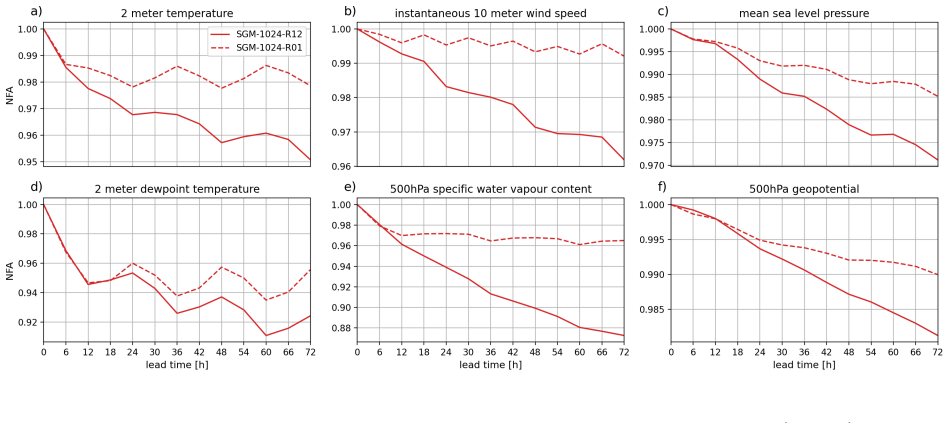
- [Abstract, Section 3.3.5, Section 5] The claim that SGM 'significantly surpasses LAM in terms of (temporal) generalisability' is stated as a general property, but the supporting evidence in Section 3.3.5 and Figure 14 is limited to 2-meter temperature at a single +6 h lead, for 512-channel models, with the advantage localized mainly over Northern Africa. No confidence intervals or effect sizes are reported for the MSE differences in Figure 14, and the text only states that results are 'similar' for the 1024-channel models without showing them. The word 'significantly' is therefore unsupported in its present form. Please either restrict the claim to the specific variable, lead time, model size, and region, or provide a multi-variable, multi-lead analysis with significance testing and with the 1024-channel results shown.
- [Sections 2.4.4, 3.3.5, and 4.3] The attribution of SGM's temporal-generalisability advantage to its global training data is not demonstrated by the extended-times experiment. The experiment varies the presence of the global domain together with at least three other differences that are known to affect model behaviour: per-variable normalization uses regional (CERRA) statistics for LAM and global (ERA5) statistics for SGM (Section 2.3); the LAM hidden grid has a fixed refinement-nine mesh extending 600 km into the boundary zone, giving higher boundary resolution than the SGM's mixed-resolution hidden grid (Section 2.2); and the SGM loss is a 25/75 regional/global weighted sum while the LAM loss is regional-only (Section 2.3). The supplementary LAM retrained on shifted times of day (Figure 14c-d) changes the training distribution but does not add global coverage, so it does not control for these confounds. The causal mechanism in Section 4.3 is therefore inferred rather than established. Please add ablation or control experiments, such as LAM trained with ERA5 normalization, SGM trained with CERRA normalization, a LAM with a coarser boundary hidden grid, or a SGM with different regional loss weights, or substantially soften the causal interpretation.
- [Sections 3.3.3, 3.3.4, and 4.1] The operational-like inference experiments are performed only with models without rollout training, while the main ideal-inference comparisons use rollout-trained models. The paper acknowledges this in Section 4.1 and notes that fine-tuning or rollout training could change the relative performance at later lead times. However, the abstract and conclusion present LAM's later-lead advantage under boundary forcing as a robust strength without carrying this caveat. Since the operational setup is the one most relevant to the recommended use cases, the conclusions about LAM's advantage in operational-like settings should either be supported by experiments with rollout-trained, fine-tuned models or be explicitly framed as applying to the non-rollout configuration used here.
minor comments (5)
- [Table 1] The CERRA available period is listed as 'Sep. 1984 - 2020'; '2020' should be 'December 2020' to be unambiguous.
- [Table A.3] The units for surface pressure and mean sea level pressure are listed as 'm s^-1'; these appear to be a copy-paste error and should be pressure units (Pa or hPa).
- [Figure 14 and Section 3.3.5] The caption and text should state the lead time, model size, and whether the displayed MSE differences were tested for significance; the current caption only identifies the model pair.
- [Reference list] Reference [33] is cited as 'Private discussions'; this is not verifiable by readers and should be replaced with a public source or removed.
- [Section 2.4.4] The extended-times experiment is described as using models without rollout training, but this is not restated in Section 3.3.5 when the results are interpreted; a brief reminder would help readers connect the experiment design to the interpretation.
Circularity Check
No circularity: benchmark conclusions rest on held-out 2020 inference, not on fitted targets or self-citation.
full rationale
This paper is an empirical inter-model benchmark rather than a derivation chain, and I find no step in which a claimed prediction or first-principles result reduces to its own inputs. The central comparisons are MSE/RMSE, skill scores, and spatial error maps computed on the 2020 test year, which was explicitly excluded from training and validation (Section 2.3: training 1984–2018, validation 2019, test 2020). The only notable tuned hyperparameter, the SGM regional/global loss weighting of 25%/75%, is described as the result of experimentation and was fixed before the test-year evaluations; it is not renamed as a prediction. The temporal-generalisability claim rests on measured SGM-versus-LAM differences at shifted initialization times (Section 3.3.5), which is an empirical outcome on unseen times, not a quantity fitted from those same scores. The Section 4.3 explanation attributing the difference to SGM's global training data is an interpretation, not an equation derived from that assumption. I also checked the self-citations: references to the Anemoi framework and prior SGM/LAM work are used to identify the platform and related methods, but the load-bearing evidence is the new held-out evaluation, not an unverified self-citation chain. The confounds noted by the skeptical reader (different normalization statistics, hidden-grid resolution over the boundary, and loss weighting) are a genuine internal-validity limitation of the comparative experiment, but they do not make the result circular: no fitted parameter, defined quantity, or cited uniqueness theorem forces the observed outcome by construction.
Assumptions & free parameters
free parameters (4)
- SGM regional loss weighting =
25% regional, 75% global
- LAM boundary domain width =
666 km
- LAM hidden grid boundary extension and resolution =
600 km extension, mesh refinement 9
- Encoder and decoder k-nearest neighbours =
12 encoder, 3 decoder
assumptions (4)
- domain assumption CERRA and ERA5 reanalyses are sufficiently accurate to serve as training targets and verification references for the regional domain.
- domain assumption The Anemoi framework's implementations fairly represent the LAM and SGM approaches.
- domain assumption The chosen ERA5 O96 (about 100 km) representation of the global and boundary domains is adequate for the regional comparison.
- standard math Standard machine-learning training assumptions (AdamW, cosine schedule, random weight initialization) apply.
Cite this review
Pith. "Pith review of A comparison of stretched-grid and limited-area modelling for data-driven regional weather forecasting." pith.science (2026). https://pith.science/paper/UOOXJASQ
@misc{pith2026250718378,
  author       = {Pith},
  title        = {Pith review of: A comparison of stretched-grid and limited-area modelling for data-driven regional weather forecasting},
  year         = {2026},
  howpublished = {\url{https://pith.science/paper/UOOXJASQ}},
  note         = {Machine review of arXiv:2507.18378}
}
read the original abstract
Regional machine learning weather prediction (MLWP) models based on graph neural networks have recently demonstrated remarkable predictive accuracy, outperforming numerical weather prediction models at lower computational costs. In particular, limited-area model (LAM) and stretched-grid model (SGM) approaches have emerged for generating high-resolution regional forecasts, based on initial conditions from a regional (re)analysis. While LAM uses lateral boundaries from an external global model, SGM incorporates a global domain at lower resolution. This study aims to understand how the differences in model design impact relative performance and potential applications. Specifically, the strengths and weaknesses of these two approaches are identified for generating deterministic regional forecasts over Europe. Using the Anemoi framework, models of both types are built by minimally adapting a shared architecture and trained using global and regional reanalyses in a near-identical setup. Several inference experiments have been conducted to explore their relative performance and highlight key differences. Results show that both LAM and SGM are competitive deterministic MLWP models with generally accurate and comparable forecasting performance over the regional domain. Various differences were identified in the performance of the models across applications. LAM is able to successfully exploit high-quality boundary forcings to make predictions within the regional domain and is suitable in contexts where global data is difficult to acquire. SGM is fully self-contained for easier operationalisation, can take advantage of more training data and significantly surpasses LAM in terms of (temporal) generalisability. Our paper can serve as a starting point for meteorological institutes to guide their choice between LAM and SGM in developing an operational data-driven forecasting system.
Figures


Figures from the paper (11 more)




Reference graph
Works this paper leans on
-
[1]
Simon Adamov et al.Building Machine Learning Limited Area Models: Kilometer-Scale Weather Fore- casting in Realistic Settings. 2025. arXiv:2504.09340 [physics.ao-ph].url:https://arxiv.org/ abs/2504.09340
arXiv 2025
-
[2]
AROME-MetCoOp: A nordic convective-scale operational weather prediction model
“AROME-MetCoOp: A nordic convective-scale operational weather prediction model”. In:Weather and Forecasting32 (2 Apr. 2017), pp. 609–627.issn: 15200434.doi:10.1175/WAF-D-16-0099.1
-
[3]
High resolution regional re-analysis ensemble for Austria
N. K. Awan et al. “High resolution regional re-analysis ensemble for Austria”. In:EGU General As- sembly. EGU24 20433. Vienna, Austria, Apr. 2024.doi:https://doi.org/10.5194/egusphere- egu24-20433
-
[4]
The HARMONIE–AROME Model Configuration in the ALADIN–HIRLAM NWP System
Lisa Bengtsson et al. “The HARMONIE–AROME Model Configuration in the ALADIN–HIRLAM NWP System”. In:Monthly Weather Review145.5 (2017), pp. 1919–1935.doi:10 . 1175 / MWR - D - 16 - 0417 . 1.url:https : / / journals . ametsoc . org / view / journals / mwre / 145 / 5 / mwr - d - 16 - 0417.1.xml
work page 2017
-
[5]
Accurate medium-range global weather forecasting with 3D neural networks
Kaifeng Bi et al. “Accurate medium-range global weather forecasting with 3D neural networks”. In: Nature619.7970 (July 2023), pp. 533–538.issn: 1476-4687.doi:10.1038/s41586-023-06185-3.url: https://doi.org/10.1038/s41586-023-06185-3
-
[6]
A foundation model for the Earth system
Cristian Bodnar et al. “A foundation model for the Earth system”. In:Nature641.8065 (May 2025), pp. 1180–1187.issn: 1476-4687.doi:10.1038/s41586- 025- 09005- y.url:https://doi.org/10. 1038/s41586-025-09005-y
doi:10.1038/s41586- 2025
-
[7]
Zied Ben Bouall` egue et al. “The Rise of Data-Driven Weather Forecasting: A First Statistical Assess- ment of Machine Learning–Based Weather Forecasts in an Operational-Like Context”. In:Bulletin of the American Meteorological Society105.6 (2024), E864–E883.doi:10.1175/BAMS- D- 23- 0162.1. url:https://journals.ametsoc.org/view/journals/bams/105/6/BAMS-D-...
doi:10.1175/bams- 2024
-
[8]
Developments in MLflow: A System to Accelerate the Machine Learning Life- cycle
Andrew Chen et al. “Developments in MLflow: A System to Accelerate the Machine Learning Life- cycle”. In:Proceedings of the Fourth International Workshop on Data Management for End-to-End Machine Learning. DEEM ’20. Portland, OR, USA: Association for Computing Machinery, 2020.isbn: 9781450380232.doi:10.1145/3399579.3399867
arXiv 2020
Show all 45 references
-
[9]
Kang Chen et al.FengWu: Pushing the Skillful Global Medium-range Weather Forecast beyond 10 Days Lead. 2023. arXiv:2304.02948 [cs.AI].url:https://arxiv.org/abs/2304.02948
2023
-
[10]
FuXi: a cascade machine learning forecasting system for 15-day global weather forecast
Lei Chen et al. “FuXi: a cascade machine learning forecasting system for 15-day global weather forecast”. In:npj Climate and Atmospheric Science6.1 (Nov. 2023), p. 190.issn: 2397-3722.doi: 10.1038/s41612-023-00512-1.url:https://doi.org/10.1038/s41612-023-00512-1
2023 doi
-
[11]
Dramsch et al.Introducing Anemoi: a new collaborative framework for ML weather forecasting
J. Dramsch et al.Introducing Anemoi: a new collaborative framework for ML weather forecasting. https://www.ecmwf.int/en/newsletter/181/news/introducing- anemoi- new- collaborative- framework-ml-weather-forecasting.doi:10.21957/de720h3x9p
-
[12]
Challenges and design choices for global weather and climate models based on machine learning
P. D. Dueben and P. Bauer. “Challenges and design choices for global weather and climate models based on machine learning”. In:Geoscientific Model Development11.10 (2018), pp. 3999–4009.doi: 10.5194/gmd-11-3999-2018.url:https://gmd.copernicus.org/articles/11/3999/2018/. 23
2018 doi
-
[13]
ECMWF.Implementation of AIFS Single v1.https : / / confluence . ecmwf . int / display / FCST / Implementation+of+AIFS+Single+v1. 2025
2025
-
[14]
ECMWF.Integrated Forecast System.url:https://www.ecmwf.int/en/forecasts/documentation- and-support/changes-ecmwf-model
-
[15]
Could Machine Learning Break the Convection Parameterization Deadlock?
P. Gentine et al. “Could Machine Learning Break the Convection Parameterization Deadlock?” In: Geophysical Research Letters45.11 (2018), pp. 5742–5751.doi:https : / / doi . org / 10 . 1029 / 2018GL078202. eprint:https://agupubs.onlinelibrary.wiley.com/doi/pdf/10.1029/2018GL078...
2018 doi
-
[16]
Tao Han et al.FengWu-GHR: Learning the Kilometer-scale Medium-range Global Weather Forecasting
-
[17]
The ERA5 global reanalysis
Hans Hersbach et al. “The ERA5 global reanalysis”. In:Quarterly Journal of the Royal Meteoro- logical Society146.730 (2020), pp. 1999–2049.doi:https : / / doi . org / 10 . 1002 / qj . 3803. eprint: https://rmets.onlinelibrary.wiley.com/doi/pdf/10.1002/qj.3803.url:https://rmets...
2020 doi
-
[18]
Regional climate downscaling over Europe : perspectives from the EURO- CORDEX community
Daniela Jacob et al. “Regional climate downscaling over Europe : perspectives from the EURO- CORDEX community”. In:REGIONAL ENVIRONMENTAL CHANGE20.2 (2020), p. 20.issn: 1436-3798.url:http://doi.org/10.1007/s10113-020-01606-9
2020 doi
-
[19]
Ryan Keisler.Forecasting Global Weather with Graph Neural Networks. 2022. arXiv:2202 . 07575 [physics.ao-ph].url:https://arxiv.org/abs/2202.07575
2022 arXiv
-
[20]
Learning skillful medium-range global weather forecasting
Remi Lam et al. “Learning skillful medium-range global weather forecasting”. In:Science382.6677 (2023), pp. 1416–1421.doi:10.1126/science.adi2336. eprint:https://www.science.org/doi/pdf/ 10.1126/science.adi2336.url:https://www.science.org/doi/abs/10.1126/science.adi2336
2023 doi
-
[21]
Simon Lang et al.AIFS – ECMWF’s data-driven forecasting system. 2024. arXiv:2406.01465 [physics.ao-ph]. url:https://arxiv.org/abs/2406.01465
2024 arXiv
-
[22]
Erik Larsson et al.Diffusion-LAM: Probabilistic Limited Area Weather Forecasting with Diffusion
-
[23]
Ilya Loshchilov and Frank Hutter.Decoupled Weight Decay Regularization. 2019. arXiv:1711.05101 [cs.LG].url:https://arxiv.org/abs/1711.05101
2019 arXiv
-
[24]
A Neural Network for Tornado Prediction Based on Doppler Radar-Derived Attributes
Caren Marzban and Gregory J. Stumpf. “A Neural Network for Tornado Prediction Based on Doppler Radar-Derived Attributes”. In:Journal of Applied Meteorology and Climatology35.5 (1996), pp. 617– 626.doi:10 . 1175 / 1520 - 0450(1996 ) 035<0617 : ANNFTP > 2 . 0 . CO ; 2.url:https ...
1996
-
[25]
A Neural Network Short-Term Forecast of Significant Thunderstorms
Donald W. McCann. “A Neural Network Short-Term Forecast of Significant Thunderstorms”. In: Weather and Forecasting7.3 (1992), pp. 525–534.doi:10.1175/1520-0434(1992)007<0525:ANNSTF> 2.0.CO;2.url:https://journals.ametsoc.org/view/journals/wefo/7/3/1520-0434_1992_007_ 0525_annst...
1992 doi
-
[26]
Ana Prieto Nemesio et al.Anemoi: A New Collaborative Framework for Data-driven Weather Fore- casting.url:https://doi.org/10.5194/egusphere-egu25-19431
-
[27]
K. P. Nielsen et al.Copernicus Arctic Regional Reanalysis (CARRA): Data User Guide - Copernicus Knowledge Base - ECMWF Confluence Wiki. Mar. 2025.url:https://confluence.ecmwf.int/ display/CKB/Copernicus+Arctic+Regional+Reanalysis+%28CARRA%29%3A+Data+User+Guide
2025
-
[28]
Thomas Nils Nipen et al.Regional data-driven weather modeling with a global stretched-grid. 2024. arXiv:2409.02891 [physics.ao-ph].url:https://arxiv.org/abs/2409.02891
2024 arXiv
-
[29]
OpenAI et al.GPT-4 Technical Report. 2024. arXiv:2303.08774 [cs.CL].url:https://arxiv.org/ abs/2303.08774
2024 arXiv
-
[30]
Joel Oskarsson, Tomas Landelius, and Fredrik Lindsten.Graph-based Neural Weather Prediction for Limited Area Modeling. 2023. arXiv:2309.17370 [cs.LG].url:https://arxiv.org/abs/2309. 17370. 24
2023 arXiv
-
[31]
Jaideep Pathak et al.FourCastNet: A Global Data-driven High-resolution Weather Model using Adap- tive Fourier Neural Operators. 2022. arXiv:2202.11214 [physics.ao-ph].url:https://arxiv. org/abs/2202.11214
2022 arXiv
-
[32]
Ilan Price et al.GenCast: Diffusion-based ensemble forecasting for medium-range weather. 2024. arXiv: 2312.15796 [cs.LG].url:https://arxiv.org/abs/2312.15796
2024 arXiv
-
[33]
2024-2025
ECMWF Machine Learning Pilot Project.Private discussions. 2024-2025
2024
-
[34]
Data-Driven Medium-Range Weather Prediction With a Resnet Pretrained on Climate Simulations: A New Model for WeatherBench
Stephan Rasp and Nils Thuerey. “Data-Driven Medium-Range Weather Prediction With a Resnet Pretrained on Climate Simulations: A New Model for WeatherBench”. In:Journal of Advances in Modeling Earth Systems13.2 (2021). e2020MS002405 2020MS002405, e2020MS002405.doi:https: //doi.o...
2021 doi
-
[35]
CERRA, the Copernicus European Regional Reanalysis system
Martin Ridal et al. “CERRA, the Copernicus European Regional Reanalysis system”. In:Quarterly Journal of the Royal Meteorological Society150.763 (2024), pp. 3385–3411.doi:https://doi.org/ 10.1002/qj.4764. eprint:https://rmets.onlinelibrary.wiley.com/doi/pdf/10.1002/qj.4764. ur...
2024 doi
-
[36]
Potential and Limitations of Machine Learning for Modeling Warm- Rain Cloud Microphysical Processes
Axel Seifert and Stephan Rasp. “Potential and Limitations of Machine Learning for Modeling Warm- Rain Cloud Microphysical Processes”. In:Journal of Advances in Modeling Earth Systems12.12 (2020). e2020MS002301 10.1029/2020MS002301, e2020MS002301.doi:https://doi.org/10.1029/ 20...
2020 doi
-
[37]
The AROME-France convective-scale operational model
Y. Seity et al. “The AROME-France convective-scale operational model”. In:Monthly Weather Review 139 (3 Mar. 2011), pp. 976–991.issn: 00270644.doi:10.1175/2010MWR3425.1
2011 doi
-
[38]
Yunsheng Shi et al.Masked label prediction: unified message passing model for semi-supervised classi- fication. 2021. arXiv:2009.03509 [cs.LG].url:https://arxiv.org/abs/2009.03509
2021 arXiv
-
[39]
Christopher Subich et al.Fixing the Double Penalty in Data-Driven Weather Forecasting Through a Modified Spherical Harmonic Loss Function. 2025. arXiv:2501.19374 [cs.LG].url:https://arxiv. org/abs/2501.19374
2025 arXiv
-
[40]
The ALADIN System and its canonical model configurations AROME CY41T1 and ALARO CY40T1
P. Termonia et al. “The ALADIN System and its canonical model configurations AROME CY41T1 and ALARO CY40T1”. In:Geoscientific Model Development11.1 (2018), pp. 257–281.doi:10.5194/gmd- 11-257-2018.url:https://gmd.copernicus.org/articles/11/257/2018/. [41]The third Met Office U...
2018 doi
-
[42]
Can Machines Learn to Predict Weather? Using Deep Learning to Predict Gridded 500-hPa Geopotential Height From Historical Weather Data
Jonathan A. Weyn, Dale R. Durran, and Rich Caruana. “Can Machines Learn to Predict Weather? Using Deep Learning to Predict Gridded 500-hPa Geopotential Height From Historical Weather Data”. In:Journal of Advances in Modeling Earth Systems11.8 (2019), pp. 2680–2693.doi:https://...
2019 doi
-
[43]
Wanghan Xu et al.ExtremeCast: Boosting Extreme Value Prediction for Global Weather Forecast
-
[45]
observation
arXiv:2402.01295 [cs.LG].url:https://arxiv.org/abs/2402.01295. 25 A Used variables Table A.3: Overview of the used variables. Prognostic variables are used as input and output and forcing variables only as input. The derived column indicates whether the variable is absent in t...
1985 arXiv
-
[2024]
arXiv:2402.00059 [cs.LG].url:https://arxiv.org/abs/2402.00059
-
[2025]
arXiv:2502.07532 [cs.LG].url:https://arxiv.org/abs/2502.07532
Reviewed August 15, 2026 · model on record in the stance chip above.
Discussion (0). Continue with ORCID to comment.